Separatrix Locator

Finding Separatrices with Deep squashed Koopman Eigenfunctions

TL;DR

Separatrices! These are boundaries between basins of attraction in dynamical systems. In high-dimensional systems like Recurrent Neural Networks, finding these boundaries can help reverse engineer their mechanism, or design optimal perturbations. But finding them is far from trivial. We recently developed a numerical method, based on approximating a Koopman Eigenfunction (KEF) of the dynamics using a deep neural network (DNN) . While this approach works, these KEFs suffer from singularities at attractors, which makes them difficult targets for DNNs to approximate. In this blogpost we explain our original method, and also improve it by using a variant we call squashed Koopman Eigenfunctions (sKEFs), which alleviate the singularities. We show how they are linked to KEFs and replicate our results from the paper.

Code: We provide a Python package implementing this method at github.com/KabirDabholkar/separatrix_locator.

Interactive version: if the interactive plots below don’t work click here.

Introduction: Fixed Points and Beyond

Many natural and artificial systems — from neural circuits making decisions to ecosystems switching between healthy and diseased states — are modelled as multistable dynamical systems. Their behaviour is governed by multiple attractors in state space, each corresponding to a stable mode of activity. Understanding these systems often boils down to understanding their geometry: where are the stable states, and how are the different basins of attraction separated?

For the last decade, a workhorse of neural circuit analysis has been fixed point analysis. By finding points where the flow vanishes and linearising around them, one can uncover local motifs underlying computation: line attractors, saddle points, limit cycles, and so on. This has yielded powerful insights into how trained RNNs implement cognitive tasks.

Finding Fixed Points

First consider a bistable dynamical system in 2 dimensions. Below is a phase-portrait of such a system, with two stable fixed points and one unstable fixed point. Click on plot to realise trajectories of the dynamics.

(click here if the plot below doesn’t load)

Trajectories converge to either one of the two fixed points. This naturally suggests an algorithm: run the dynamics from many initial conditions to find the stable fixed points.

Now try to click somewhere that will lead you exactly to the saddle point. Did you succeed? It’s almost impossible.

This motivates developing a principled way to find such points. One solution is to define a specific scalar function of the dynamics whose only minima are given by all the fixed points. One such function is the kinetic energy \(q(\boldsymbol x)=\frac{1}{2}\Vert f(\boldsymbol x)\Vert^2\) . By differentiating this function, one can perform gradient descent to find these minima. The interactive plot below realises such trajectories.

(click here if the plot below doesn’t load)

Now we can find both stable and unstable fixed points. Linearising around the fixed points provides an interpretable approximation of the dynamics in the neighbourhood of those points. Several works adopt this approach of fixed point finding to reverse-engineer either task-trained or data-trained RNNs .

But fixed points are only half the story.

When a system receives a perturbation — for example, a sensory input or an optogenetic pulse — the key question is often not where it started, but which side of the separatrix it ends up on. The separatrix is the boundary in state space separating different basins of attraction. Crossing it means switching decisions, memories, or ecological states. Failing to cross means staying put. For high-dimensional systems, these boundaries are typically nonlinear, curved hypersurfaces, invisible to fixed points and local linearisations around them.

What if we could learn a single smooth scalar function whose zero level set is the separatrix?

Below is an example of such a function that we constructed for this simple system (click on it to run trajectories).

(click here if the plot below doesn’t load)

Our main contribution is a numerical method to approximate such functions using deep neural networks in order to find separatrices in multistable dynamical systems in high-dimensions.

Setting

We consider autonomous dynamical flows of the form:

\[\begin{equation} \dot{\boldsymbol{x}} = f(\boldsymbol{x}) \label{eq:ODE} \end{equation}\]

governing the state \(\boldsymbol{x} \in \mathbb R^N\), where \(\dot \square\) is shorthand for the time derivative \(\frac{d}{dt}\square\) and \(f: \mathbb R^N \to \mathbb R^N\) defines the dynamical flow.

The Goal:
Find a smooth scalar function \(\psi:\mathbb{R}^N\to\mathbb{R}\) that grows as we move away from the separatix, i.e., \(\psi(\boldsymbol x)=0\) for \(x\in\text{separatrix}\) and grows as it moves away from the separatrix.

The Sandwich of Bistability

Any bistable system can be decomposed as follows: it will have two attractors, their respective basins of attraction and the separatrix between them. This is like a cheese sandwich: the attractors are slices of bread, and the separatrix is the slice of cheese between them. We can call this the Sandwich of Bistability. In general, this sandwich could be arbitrarily oriented in \(\mathbb R^N\) and even nonlinearly warped.

The Sandwich of Bistability: Two attractors and their basins of attraction (bread slices) separated by a separatrix (cheese slice). We only care about mapping the coordinates along bistable axis.

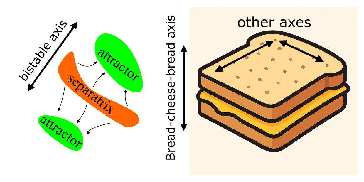
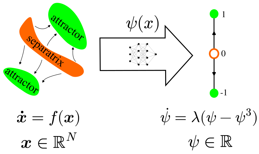
With our scalar function \(\psi:\mathbb{R}^N\to\mathbb{R}\) we would like to perform a special type of dimensionality reduction: we only care to identify our location along the attractor–separatrix–attractor axis, i.e., along the depth of sandwich.

One way to achieve this is to have this scalar observable \(\psi(\boldsymbol x)\) imitate the bistable dynamics along this axis. Thus we pick a simple example of bistable dynamics in 1D (hover your cursor over it to see the plot):

$$ \begin{equation} \dot \psi = \lambda (\psi-\psi^3) \label{eq:sKEFsimple} \end{equation} $$

with \(\lambda>0\), dropping the \(\boldsymbol x\) notation for a moment for clarity. This system has fixed point attractors at \(\pm 1\) and an unstable fixed point (a separatrix) at \(0\) – a 1D Sandwich of Bistability.

Mapping the high-D state to a 1D bistable system.

Now we want to couple the \(\psi\) dynamics with the \(\boldsymbol x\) dynamics so we bring back the \(\boldsymbol x\) dependence. Specifically as \(\boldsymbol x(t)\) evolves in time according to \(\eqref{eq:ODE}\):

\[\begin{equation} \frac{d}{dt}\bigg(\psi\big(\boldsymbol{x}(t)\big)\bigg) = \lambda\bigg[\psi\big(\boldsymbol{x}(t)\big) - \psi\big(\boldsymbol{x}(t)\big)^3\bigg]. \label{eq:sKEF} \end{equation}\]

This means that if we were to observe the value of \(\psi(\boldsymbol x)\) as \(\boldsymbol x\) evolved in time, that value would evolve according \(\eqref{eq:sKEFsimple}\).

It seems that finding solutions to \(\eqref{eq:sKEF}\) could be the key to constructing a separatrix locator. The value \(\psi(\boldsymbol x)\) would be the coordinate of \(\boldsymbol x\) along the bistable axis. This value would be \(0\) when \(\boldsymbol x\) is anywhere on the separatrix, exactly our stated goal.

(squashed) Koopman Eigenfunctions

At this stage, it’s worth noticing that the left hand side of \(\eqref{eq:sKEF}\) is actually a known object called the Lie derivative of \(\psi\) along the flow given by \(f\), and also known as the infinitesimal generator of the Koopman operator, (See ).

To make this link explicit, we first define the propagator function \(F_\tau(x(t)):=x(t+\tau)\) where \(x(t)\) is any solution to \(\eqref{eq:ODE}\). The Koopman operator \(\mathcal K_\tau\) is defined as

\[\mathcal K_\tau g = g \circ F_\tau\]

where \(g\) is any\(g\) must belong to a Hilbert space, meaning that it must come with inner product (and it's associated norm), e.g., $$\langle f,g\rangle:=\int_{\mathbb R^N}f(\boldsymbol x)g(\boldsymbol x)d\boldsymbol x$$ thus requiring that the function be square integrable. scalar function of the state-space \(\mathbb R^N\). Its infinitesimal generator \(\mathcal K\) (dropping the subscript) is essentially a time-derivative:

\[\begin{equation} \mathcal Kg = \lim_{\tau\to0} \frac{\mathcal K_\tau g - g}{\tau} =\lim_{\tau\to0} \frac{g\circ F_\tau - g}{\tau} = \frac{d}{d\tau} g \circ F_\tau\bigg\vert_{\tau=0}. \label{eq:koopman_generator} \end{equation}\]

The last version if evaluated on a trajectory \(x(t)\) is the left hand side of \(\eqref{eq:sKEF}\), allowing us to rewrite it compactly as

\[\begin{equation} \mathcal K\psi = \lambda (\psi-\psi^3). \label{eq:sKEF_compact} \end{equation}\]

This equation is almost an eigenfunction equation. All we need is to drop the cubic term:

\[\begin{equation} \mathcal K\phi = \lambda \phi. \label{eq:KEF} \end{equation}\]

In fact, the two problems are closely related. We can show that solutions to \(\eqref{eq:KEF}\) can be transformed into solutions of \(\eqref{eq:sKEF_compact}\) and vice versa by squashing and unsquashing. If \(\phi\) is a solution to \(\eqref{eq:KEF}\), then we can obtain a solution \(\psi\) to \(\eqref{eq:sKEF_compact}\) via:

\[\begin{equation} \psi(\boldsymbol{x}) = \frac{ \phi(\boldsymbol{x})}{ \sqrt{1+\phi(\boldsymbol{x})^2} } \label{eq:squash} \tag{squash} \end{equation}\]

Conversely, if \(\psi\) is a solution to \(\eqref{eq:sKEF_compact}\), then we can obtain a solution \(\phi\) to \(\eqref{eq:KEF}\) via:

\[\begin{equation} \phi(\boldsymbol{x}) = \frac{ \psi(\boldsymbol{x})}{ \sqrt{1-\psi(\boldsymbol{x})^2} } \label{eq:unsquash} \tag{unsquash} \end{equation}\]

We provide an informal derivation.

Derivation: From eigenfunction to squashed eigenfunction and back

To do this, define the pointwise transforms \(\psi \;=\; u(\phi) \;:=\; \frac{\phi}{\sqrt{1+\phi^2}}, \qquad \phi \;=\; v(\psi) \;:=\; \frac{\psi}{\sqrt{1-\psi^2}}.\)

---

First we will derive useful identity: the chain rule for the Koopman generator.

Koopman chain rule

Let \(\phi:\mathbb R^N \to \mathbb R\) be a smooth scalar observable, and let \(u:\mathbb R \to \mathbb R\) be a smooth scalar nonlinearity. Let \(\psi(\boldsymbol x) = u(\phi(\boldsymbol x)).\)

The Koopman generator is

\[\mathcal K g(\boldsymbol x) = \nabla g(\boldsymbol x)\cdot f(\boldsymbol x),\]

for any \(g\) where \(f(\boldsymbol x)\) is the underlying vector field.

By the multivariable chain rule for gradients,

\[\nabla \psi(\boldsymbol x) = u'\big(\phi(\boldsymbol x)\big)\,\nabla \phi(\boldsymbol x).\]

Applying the Koopman generator gives

\[\mathcal K \psi(\boldsymbol x) = \nabla \psi(\boldsymbol x)\cdot f(\boldsymbol x) = u'\big(\phi(\boldsymbol x)\big)\,\nabla \phi(\boldsymbol x)\cdot f(\boldsymbol x) = u'\big(\phi(\boldsymbol x)\big)\,\mathcal K \phi(\boldsymbol x).\]

Therefore, for any smooth \(u\) and \(\phi\),

\[\boxed{\;\mathcal K[u(\phi)] = u'(\phi)\,\mathcal K\phi\; }.\]

---

From \(\mathcal K\phi=\lambda\phi\) to \(\mathcal K\psi=\lambda(\psi-\psi^3)\)

Assume \(\mathcal K\phi \;=\; \lambda \phi.\)

Recall that \(\psi = u(\phi)\) where \(u(z)=\dfrac{z}{\sqrt{1+z^2}}\). Compute \(u'(z)\):

\[\begin{align*} u'(z) &= (1+z^2)^{-\frac{1}{2}} + z\cdot\Big(-\frac{1}{2}\Big)(1+z^2)^{-\frac{3}{2}}\cdot (2z) \\[2pt] &= (1+z^2)^{-\frac{1}{2}} - z^2(1+z^2)^{-\frac{3}{2}} \\[2pt] &= \frac{1+z^2-z^2}{(1+z^2)^{\frac{3}{2}}} \\[2pt] &= \frac{1}{(1+z^2)^{\frac{3}{2}}} \end{align*}\]

By the Koopman chain rule,

\[\mathcal K\psi \;=\; u'(\phi)\,\mathcal K\phi \;=\; \frac{1}{(1+\phi^2)^{3/2}}\,\lambda\phi \;=\; \lambda\,\frac{\phi}{(1+\phi^2)^{3/2}}.\]

But

\[\psi - \psi^3 = \frac{\phi}{\sqrt{1+\phi^2}} - \frac{\phi^3}{(1+\phi^2)^{3/2}} = \frac{\phi(1+\phi^2)-\phi^3}{(1+\phi^2)^{3/2}} = \frac{\phi}{(1+\phi^2)^{3/2}}.\]

Hence \(\boxed{\;\mathcal K\psi \;=\; \lambda(\psi-\psi^3)\; }.\)

---

From \(\mathcal K\psi=\lambda(\psi-\psi^3)\) back to \(\mathcal K\phi=\lambda\phi\)

Assume \(\mathcal K\psi \;=\; \lambda(\psi-\psi^3).\)

Recall that \(\phi = v(\psi)\) where \(v(z)=\dfrac{z}{\sqrt{1-z^2}}\). Compute \(v'(z)\):

\[\begin{align*} v'(z) &= (1-z^2)^{-\frac{1}{2}} + z\cdot\frac{1}{2}(1-z^2)^{-\frac{3}{2}}\cdot (2z) \\[2pt] &= (1-z^2)^{-\frac{1}{2}} + z^2(1-z^2)^{-\frac{3}{2}} \\[2pt] &= \frac{1}{(1-z^2)^{\frac{3}{2}}} \end{align*}\]

Apply the Koopman chain rule with \(\phi=v(\psi)\):

\[\mathcal K\phi \;=\; v'(\psi)\,\mathcal K\psi \;=\; \frac{1}{(1-\psi^2)^{3/2}}\,\lambda(\psi-\psi^3) \;=\; \lambda\,\frac{\psi(1-\psi^2)}{(1-\psi^2)^{3/2}} \;=\; \lambda\,\frac{\psi}{\sqrt{1-\psi^2}} \;=\; \lambda\,\phi.\]

Thus \(\boxed{\;\mathcal K\phi \;=\; \lambda \phi\; }.\)

---

Conclusion

The pointwise transforms \(\psi = u(\phi) = \frac{\phi}{\sqrt{1+\phi^2}}, \qquad \phi = v(\psi) = \frac{\psi}{\sqrt{1-\psi^2}}\)

carry solutions of the linear Koopman eigenfunction equation to solutions of the cubic equation and back: \(\mathcal K\phi=\lambda\phi \quad\Longleftrightarrow\quad \mathcal K\psi=\lambda(\psi-\psi^3).\)

Note that this derivation is highly non-rigorous. We gloss over the square integrability of \(\psi\) and \(\phi\), and even whether they are defined everywhere in \(\mathbb R^N\). According to our sandwich of bistability, we expect \(\psi(\boldsymbol {x^*})=\pm1\) at the attractors. According to \(\eqref{eq:unsquash}\), \(\phi(\boldsymbol {x^*})=\pm\infty\),

Enter Deep Neural Networks

Now that we know the properties of the desired \(\psi\), it’s time to find it. So how do we solve the \(\eqref{eq:sKEF}\) for a high-dimensional nonlinear system. This is where deep neural networks (DNNs) come in…

First we re-write \(\eqref{eq:sKEF}\) as a partial differential equation (PDE):

\[\begin{equation} \nabla_{\boldsymbol{x}}\psi(\boldsymbol{x}) \cdot f(\boldsymbol{x}) = \lambda[\psi(\boldsymbol{x}) - \psi(\boldsymbol{x})^3], \label{eq:sKEFPDE} \end{equation}\]

recognising that \(\mathcal Kg=\nabla g \cdot f\) is another way to write the Koopman generator, using the multivariate chain rule on \(\eqref{eq:koopman_generator}\). This PDE means that instead of running the ODE \(\eqref{eq:ODE}\) to get trajectories \(\boldsymbol x(t)\), we can instead leverage the ability of DNNs to solve PDEs.

We formulate a mean squared error loss for PDE \(\eqref{eq:sKEFPDE}\):

\[\begin{equation} \mathcal{L}_{\text{PDE}} = \mathbb{E}_{\boldsymbol{x} \sim p(\boldsymbol{x})} \Bigg[ \nabla \psi(\boldsymbol{x}) \cdot f(\boldsymbol{x}) - \lambda \Big(\psi(\boldsymbol{x})-\psi(\boldsymbol{x})^3\Big) \Bigg]^2, \label{eq:pde_loss} \end{equation}\]

where \(p(\boldsymbol{x})\) is a distribution over the phase space . We can now parameterise \(\psi\) using a DNN, and train its weights to optimise \(\eqref{eq:pde_loss}\). This gradient-based PDE formulation is particularly convenient for implementation with DNNs since we can leverage automatic differentiation to compute the gradients efficiently. DNNs are also used in this way in physics-informed neural networks , encouraging DNNs to satisfy known physics, e.g., Navier–Stokes PDEs.

Naturally, this doesn’t work out of the box. There are quite a few challenges – some common to eigenvalue problems, and some unique to our setting. You can click on them to find out more about why they arise, and how we solve them.

Trivial solutions

As with any eigenvalue problem, this loss admits the trivial solution \(\psi \equiv 0\). To discourage such solutions, we introduce a shuffle-normalization loss where the two terms are sampled independently from the same distribution:

\[\begin{equation} \mathcal{L}_{\text{shuffle}} = \mathbb{E}_{\boldsymbol{x} \sim p(\boldsymbol{x}), \tilde{\boldsymbol{x}} \sim p(\boldsymbol{x})} \Bigg[ \nabla \psi(\boldsymbol{x}) \cdot f(\boldsymbol{x}) - \lambda \Big(\psi(\tilde{\boldsymbol{x}}) - \psi(\tilde{\boldsymbol{x}})^3\Big) \Bigg]^2, \end{equation}\]

and optimise the ratio:

\[\begin{equation}\mathcal{L}_{\text{ratio}} = \frac{\mathcal{L}_{\text{PDE}}}{\mathcal{L}_{\text{shuffle}}}. \label{eq:ratio loss} \end{equation}\]

Degeneracy across basins

Koopman eigenfunctions (KEFs) have an interesting property: a product of two KEFs is also a KEF. This can be seen by applying the PDE to the product of two such functions

\[\begin{equation} \nabla[\phi_1(x)\phi_2(x)] \cdot f(x) = (\lambda_1 + \lambda_2) \phi_1(x)\phi_2(x). \end{equation}\]

We’ll soon see that this translates to squashed KEFs as well. First, consider a smooth KEF \(\phi^1\) with \(\lambda = 1\) that vanishes only on the separatrix (what we want). Now, consider a piecewise-constant function \(\phi^0\) with \(\lambda = 0\) that is equal to 1 on one basin, and zero on another basin. The product \(\phi^1 \phi^0\) remains a valid KEF with \(\lambda = 1\), but it can now be zero across entire basins—thereby destroying the separatrix structure we aim to capture. Because of the relation between KEFs and sKEFs, this problem carries over to our squashed case. To mitigate this problem, we add another regulariser that causes the average value of \(\psi\) to be zero, encouraging negative and positive values on both sides of the separatrix.

Degeneracy in high dimensions

If the flow itself is separable, there is a family of KEFs that can emphasise one dimension over the others. Consider a 2D system \(\dot{x} = f_1(x), \quad \dot{y} = f_2(y)\), and the KEFs \(A(x)\) and \(B(y)\). There is a family of valid solutions \(\psi(x, y) = A(x)^{\mu} B(y)^{1 - \mu}\), for \(\mu \in R\).

If \(\mu=0\) for instance, the \(x\) dimension is ignored. To mitigate this, we choose distributions for training the DNN that emphasise different dimensions, and then combine the results.

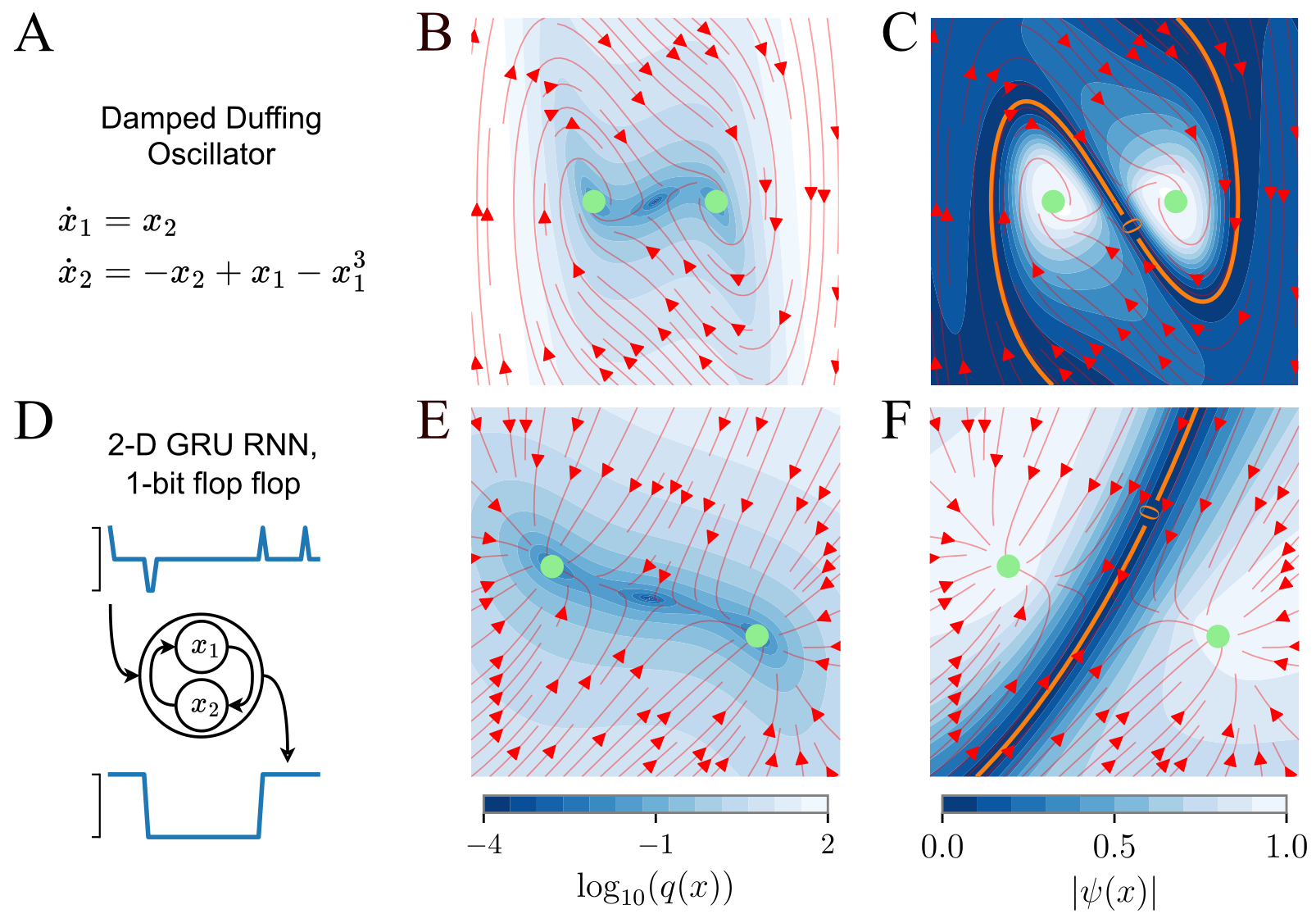
Does It Work?

Now that we know what we are looking for (PDE equation), and how to find it (DNN), let’s put it all together. We train a DNN on a bistable damped oscillator, and on a 2D GRU trained on a 1-bit flip-flop task. In both cases, the resulting \(\psi\) has a zero level set on the separatrix.

A: ODEs for the damped duffing oscillator. B: Kinetic energy function identifies stable and unstable fixed points. C: DNN approximation of the sKEF and it's level sets. The zero-level set (orange) aligns with the separatrix. D,E,F: Same for a 2D GRU RNN trained on a 1-bit flip flop task.

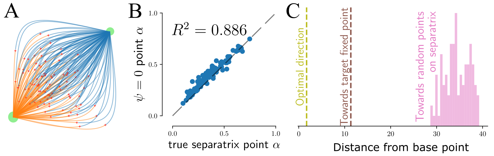
Finally, we take a published \(N=668\) unit RNN trained to reproduce the activity of neurones from anterior lateral motor cortex of mice trained to respond to optogenetic stimulation of their somatosensory cortex . By simulating the RNN we can locate the two attractors. The separatrix is an \((N-1)\)-dimensional manifold in \(\mathbb{R}^N\). To evaluate our method, we sample this high-D space by drawing random cubic Hermite curves that connect the two attractors (Fig. A). We then run many simulations via a binary-search along each curve (parameterised by \(\alpha\in[0,1]\)) to find the true separatrix crossing, and compare with \(\psi=0\), finding close agreement (Fig. B). This also allows us to design optimal perturbations. If we want to change the network’s decision, pushing the system towards the desired attractor may not be the most efficient direction. Using \(\psi\), we design minimal perturbations that cross the separatrix. The resulting perturbation size is smaller than perturbations aimed at the target fixed point or random separatrix locations (Fig. C).

A: Hermite curves connecting attractors of a data-trained RNN (2D projection from 668D) with true separatrix points (red). B: sKEF zeroes versus true separatrix points along each curve. C: Norm of perturbations to reach separatrix from base point $\boldsymbol{x}_\text{base}$.

Summary and Outlook

Making sense of high-dimensional dynamical systems is not trivial. We added another tool to the toolbox – a separatrix finder. More generally, one can think of our cubic \(\eqref{eq:sKEFsimple}\) as a normal form for bistability. This is a canonical, or simple, version of a dynamical system with the same topology. Our method allows to reduce the high-D dynamics into such a form. In the future, we hope to extend this to many more applications. Check out our code and apply it to your own dynamical systems. Feel free to reach out to us, we’re excited to help and learn about new applications!