JEPA as a Neural Tokenizer: Learning Robust Speech Representations with Density Adaptive Attention
A two-stage self-supervised framework combining Joint-Embedding Predictive Architecture with density-adaptive attention for efficient speech tokenization and reconstruction through mixed-radix quantization
* Work does not relate to position at Amazon.
Hybrid Discrete-Continuous Speech Representations via JEPA with Density Adaptive Attention
Overview
We introduce a two-stage self-supervised learning framework that combines Joint-Embedding Predictive Architecture (JEPA)
Key innovation: By integrating Density Adaptive Attention-based gating (i.e. Gaussian Mixture gating)
Motivation: Why JEPA for Speech?
Traditional speech codec training couples representation learning with reconstruction objectives, forcing the encoder to prioritize features that minimize waveform-level losses. This conflates two distinct goals:
- Learning semantically meaningful representations that capture linguistic and acoustic structure
- Preserving perceptual quality for high-fidelity reconstruction
JEPA addresses this by separating concerns: the encoder learns to predict masked representations in latent space (Stage 1), then a separate decoder learns to map these representations to audio (Stage 2). This architectural separation enables:
- Better representations: Encoder optimizes for semantic content rather than low-level waveform details
- Efficiency: Fine-tuning encoder reduces Stage 2 training cost
- Flexibility: Same encoder can support multiple downstream tasks (Text-To-Speech, Voice Conversion, Automatic Speech Recognition etc.)
- Scalability: Stage 1 can leverage large unlabeled datasets
The integration of DAAM enhances this framework by introducing adaptive attention that learns which temporal regions and features are most informative for prediction, naturally discovering speech-relevant patterns.
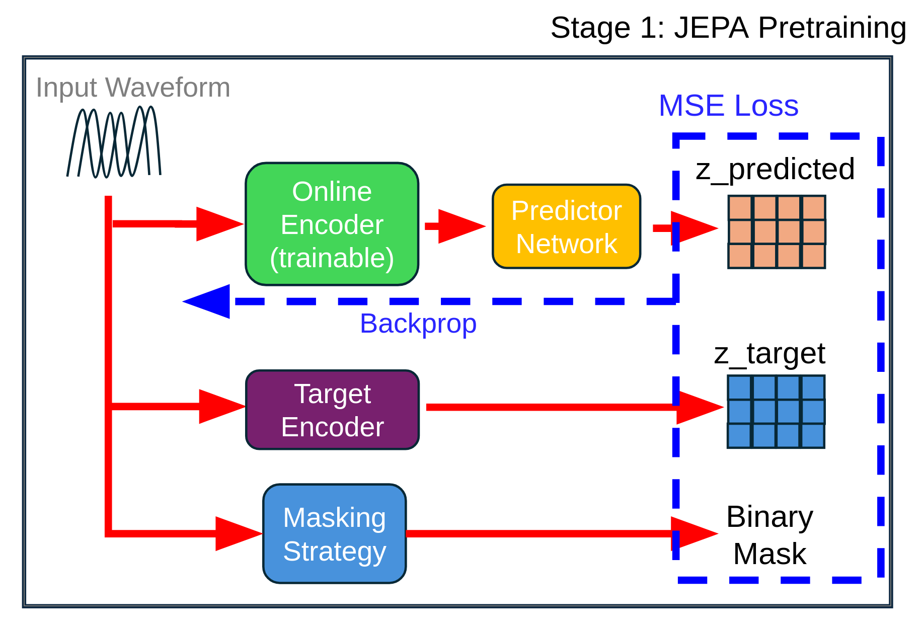
Stage 1: Self-Supervised JEPA Encoder with DAAM
JEPA Masking Strategy
The JEPA framework employs block-based temporal masking to create a self-supervised learning objective. For a batch of audio sequences with temporal length $T$, binary masks $\mathbf{m} \in {0,1}^{B \times T}$ are generated, where $1$ indicates visible (context) regions and $0$ indicates masked (target) regions.
Block Masking Algorithm:
Given mask ratio $\rho \in [0,1]$, minimum span length $s_{\text{min}}$, and maximum span length $s_{\text{max}}$, we construct masks as follows:
-
Initialize: $\mathbf{m} \leftarrow \mathbf{1}_{B \times T}$ (all positions visible)
- For each sample $b \in {1, \ldots, B}$:
- Compute target: $n_{\text{mask}} = \lfloor \rho \cdot T \rfloor$
- Initialize counter: $n_{\text{masked}} \leftarrow 0$
- While $n_{\text{masked}} < n_{\text{mask}}$:
- Sample span length: $\ell \sim \text{Uniform}(s_{\text{min}}, s_{\text{max}})$
- Sample start position: $t_{\text{start}} \sim \text{Uniform}(0, T - \ell)$
- Compute end position: $t_{\text{end}} \leftarrow \min(t_{\text{start}} + \ell, T)$
- Set mask: $\mathbf{m}[b, t] \leftarrow 0$ for all $t \in [t_{\text{start}}, t_{\text{end}})$
- Update counter: $n_{\text{masked}} \leftarrow n_{\text{masked}} + (t_{\text{end}} - t_{\text{start}})$
- Return: Mask tensor $\mathbf{m}$
This block masking strategy creates contiguous masked spans rather than random individual positions. Block masking forces the model to learn longer-range temporal dependencies and semantic content.
Masking hyperparameters in our implementation:
- Mask ratio: $\rho = 0.5$ (50% of timesteps masked)
- Minimum span: $s_{\text{min}} = 2$ frames
- Maximum span: $s_{\text{max}} = T/4$ frames (adaptive to sequence length)
At 2.5 Hz frame rate, this corresponds to variable spans adapted to the sequence length.
Density Adaptive Attention for Temporal Feature Modulation
The core innovation integrating a stabilized version of the original DAAM into JEPA is the DensityAdaptiveAttention module, which computes adaptive attention gates based on learned Gaussian mixture distributions. Unlike standard self-attention that computes pairwise dot-product between positions, DAAM learns to identify statistically salient temporal regions based on their distribution characteristics.
Mathematical Formulation:
For input features $\mathbf{x} \in \mathbb{R}^{B \times C \times T}$ (batch size, channels, time), the DAAM module operates along the temporal axis as follows:
Step 1: Compute temporal statistics
For each batch and channel, compute the mean and variance across time:
\[\mu = \frac{1}{T}\sum_{t=1}^T x_{:,:,t} \in \mathbb{R}^{B \times C \times 1}\] \[\sigma^2 = \frac{1}{T}\sum_{t=1}^T (x_{:,:,t} - \mu)^2 \in \mathbb{R}^{B \times C \times 1}\]These statistics capture the distributional properties of temporal features at each channel.
Step 2: Define learnable Gaussian parameters
For $K$ Gaussian components, we maintain learnable parameters:
- Mean offsets: $\boldsymbol{\delta} = [\delta_1, \ldots, \delta_K] \in \mathbb{R}^K$
- Initialized to: $\delta_k = 0.0$ for all $k$
- Allows shifting the center of each Gaussian component
- Log-scale parameters: $\boldsymbol{\nu} = [\nu_1, \ldots, \nu_K] \in \mathbb{R}^K$
- Initialized to: $\nu_k = \log(0.5)$ for all $k$
- Transformed via softplus for positivity
The scale parameters are computed as:
\[\tilde{\sigma}_k = \text{softplus}(\nu_k) + \epsilon = \log(1 + \exp(\nu_k)) + \epsilon\]where $\epsilon = 10^{-3}$ ensures numerical stability and prevents collapse to zero variance.
Step 3: Compute standardized deviations for each Gaussian
For each component $k \in {1, \ldots, K}$ and each timestep $t$:
\[z_{k,t} = \frac{x_{:,:,t} - (\mu + \delta_k)}{\sigma \cdot \tilde{\sigma}_k + \epsilon}\]This computes how many “standard deviations” (scaled by $\tilde{\sigma}_k$) each timestep is from the adjusted mean $\mu + \delta_k$.
Step 4: Evaluate log-probability density under each Gaussian
For each component $k$, the log-probability density at each timestep is:
\[\log p_k(x_t) = -\frac{1}{2}z_{k,t}^2 - \log \tilde{\sigma}_k - \frac{1}{2}\log(2\pi)\]This is the standard Gaussian log-density formula applied to the standardized deviations. The three terms represent:
- Squared Mahalanobis distance: $-\frac{1}{2}z_{k,t}^2$
- Scale normalization: $-\log \tilde{\sigma}_k$
- Constant normalization: $-\frac{1}{2}\log(2\pi)$
Step 5: Aggregate Gaussian components via log-sum-exp
To form a mixture of Gaussians, we aggregate the log-probabilities:
\[\log \mathbf{G}(x_t) = \text{logsumexp}(\{\log p_1(x_t), \ldots, \log p_K(x_t)\}) - \log K\]where the log-sum-exp operation is:
\[\text{logsumexp}(\mathbf{a}) = \log \sum_{k=1}^K \exp(a_k)\]computed in a numerically stable manner. The $-\log K$ term normalizes the mixture to have equal prior weights on all components.
Step 6: Compute attention gate and modulate features
The final attention gate is obtained by exponentiating the log-density:
\[\mathbf{G}(x_t) = \exp(\log \mathbf{G}(x_t))\]The output features are then:
\[\mathbf{y}_t = \mathbf{x}_t \odot \mathbf{G}(x_t)\]where $\odot$ denotes element-wise multiplication. DAAM operates on a learned 1-channel attention projection over time: features are first projected to a single channel, the Gaussian mixture gate is computed on that 1D temporal signal, and the resulting gate scales the full feature tensor.
Implementation details:
- All computations performed in FP32 for numerical stability
- Clamping applied to variance ($\text{var} \geq 10^{-6}$) to prevent NaN
- Softplus transformation ensures positive scales: $\tilde{\sigma}_k > 0$
- Number of Gaussians: $K = 4$ across all layers
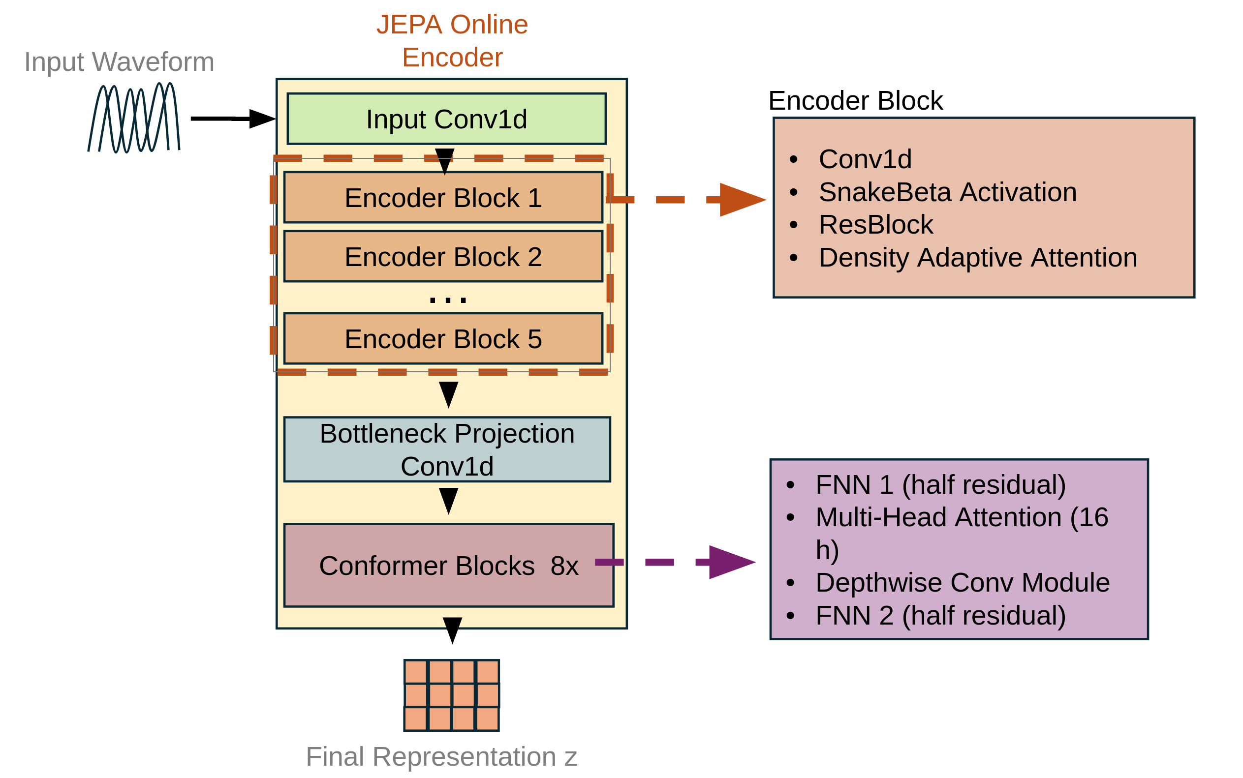
JEPA Encoder Architecture
The JEPA encoder consists of two parallel pathways that share weights but serve different roles:
1. Context Encoder (Online Network)
- Processes the full audio input
- Masking is applied later in feature space by replacing hidden timesteps with a learned mask token before the predictor
- Parameters updated via gradient descent
2. Target Encoder (EMA Network)
- Processes the full audio input
- Provides stable targets for prediction
- Parameters updated via exponential moving average (EMA)
Architecture details:
Each encoder follows a convolutional-transformer hybrid design:
Downsampling path:
Input raw waveform [B, 1, T_wav] passes through Conv1D blocks with stride, progressing through channel dimensions: 64→128→256→384→512→512. The total stride is 8×8×5×5×6 = 9600 samples/hop at 24kHz, resulting in a latent representation [B, 512, T_z] where T_z corresponds to approximately 2.5 Hz frame rate.
Conformer blocks
- 8 Conformer layers with 16 attention heads
- Each layer: Self-attention → Feedforward → Convolution → LayerNorm
- DAAM gating is applied in the encoder blocks (after the strided conv + residual stacks); there is no DAAM after the Conformer blocks in this repo.
Integration with DAAM:
After each Conformer block, features pass through GAttnGateG modules that implement the following operations:
- Project features to single channel via 1×1 convolution
- Compute DAAM gate from projected features
- Apply learned scaling: $\mathbf{y} = \mathbf{x} \cdot (1 + \alpha \cdot \text{gate})$
- Parameter $\alpha$ (initialized to 0.05) controls modulation strength
This adaptive gating mechanism allows the model to emphasize or suppress features at different temporal positions based on their statistical properties.
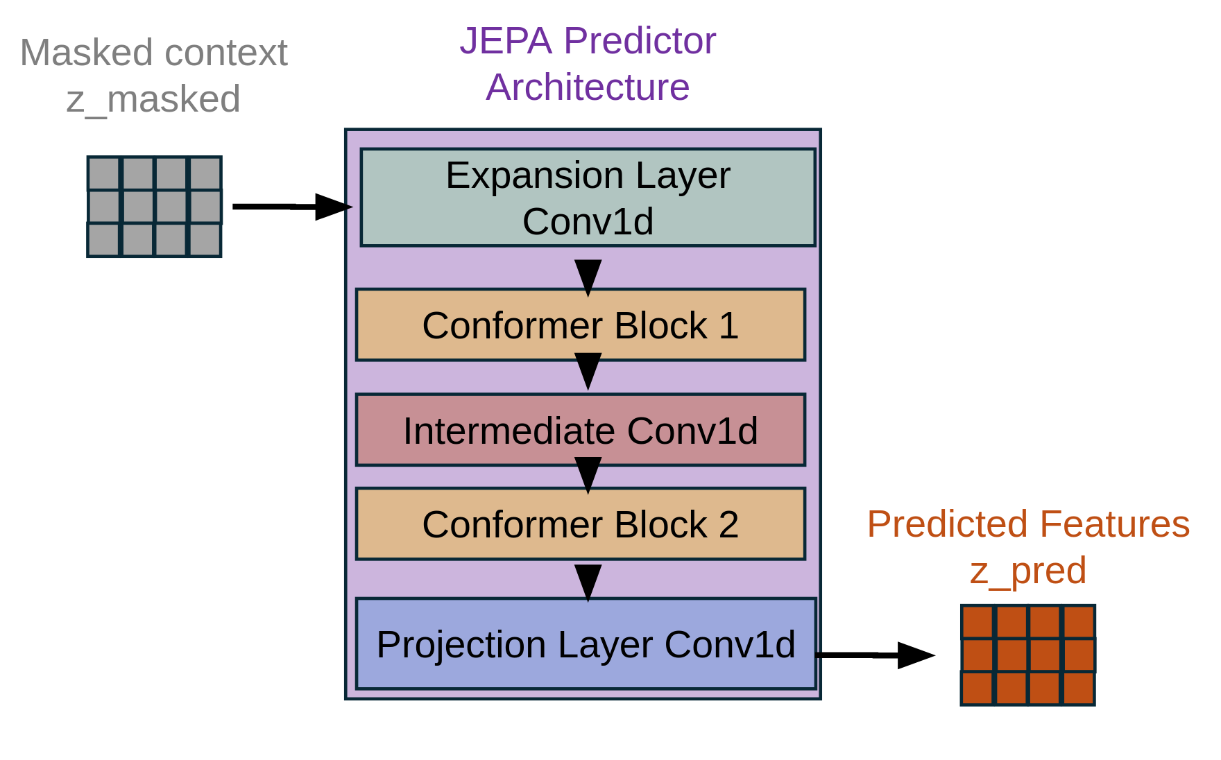
JEPA Predictor Network:
The predictor takes context representations and predicts masked regions. The predictor uses two Conformer blocks; the number of attention heads is 16. That processes the masked context features and outputs predictions for all temporal positions. The predictor only receives context (visible) regions but must predict features at all positions. The mask is applied to the loss calculation.
Stage 1 Training Objective
The JEPA training objective is pure self-supervised prediction in latent space:
Loss Function:
\[\mathcal{L}_{\text{JEPA}} = \frac{1}{N_{\text{mask}} \cdot C} \sum_{t \in \mathcal{M}} \| \mathbf{z}_{\text{pred}}^{(t)} - \text{sg}(\mathbf{z}_{\text{target}}^{(t)}) \|^2\]where:
- $\mathcal{M} = {t : m_t = 0}$ is the set of masked positions
- $N_{\mathrm{mask}} = \lvert \mathcal{M} \rvert$ is the number of masked timesteps
- $C$ is the channel dimension
- $\text{sg}(\cdot)$ denotes stop-gradient operation on target features
- $\mathbf{z}_{\text{pred}}^{(t)} \in \mathbb{R}^C$ is the predictor output at position $t$
- $\mathbf{z}_{\text{target}}^{(t)} \in \mathbb{R}^C$ is the target encoder output at position $t$
Implementation:
The mask is created with 1 indicating visible positions and 0 indicating masked positions. During training, the loss is computed only on the masked regions by weighting the squared differences. The numerator sums the squared errors across all masked positions and channels, while the denominator normalizes by the number of masked tokens multiplied by the channel dimension, ensuring proper scaling regardless of mask ratio.
Key properties:
- Masked-only prediction: Loss computed only on masked regions $\mathcal{M}$
- Stop-gradient on target: Target encoder provides fixed targets
- Proper normalization: Loss normalized by number of masked tokens × channels
- No reconstruction: Never reconstructs waveform in Stage 1
EMA Target Update:
After each training step, the target encoder parameters are updated via exponential moving average:
\[\boldsymbol{\theta}_{\text{target}} \leftarrow \tau \boldsymbol{\theta}_{\text{target}} + (1-\tau) \boldsymbol{\theta}_{\text{online}}\]where $\tau = 0.996$ is the momentum coefficient.
Training hyperparameters:
- Optimizer: AdamW with $\beta_1 = 0.8$, $\beta_2 = 0.99$
- Learning rate: $1.5 \times 10^{-4}$
- Weight decay: $10^{-3}$
- Batch size: 32
- Max audio length: 15 seconds @ 24kHz
- Training steps: 24,000
Collapse monitoring (no gradient):
To detect potential representation collapse, we monitor (without backpropagation) the standard deviation of predictor outputs across batch and temporal dimensions. If the mean standard deviation falls below 0.01, a warning is logged. This monitoring helps detect if the predictor outputs collapse to constant values, but does NOT contribute to the loss.
Stage 2: Fine-tuning Encoder + FSQ Quantization + HiFi-GAN Decoder
After Stage 1 completes, the JEPA encoder weights are fine-tuned and used as a feature extractor for Stage 2 training. Stage 2 introduces quantization and waveform reconstruction.
Finite Scalar Quantization (FSQ)
FSQ provides efficient discrete tokenization without requiring codebook learning
FSQ Formulation:
For latent features $\mathbf{z}_e \in \mathbb{R}^{B \times C \times T}$ from the encoder, FSQ quantizes each dimension independently:
Given levels $\mathbf{L} = [L_1, \ldots, L_D]$ where $D$ divides $C$:
-
Project to quantization space: \(\mathbf{z}_e^{\prime} = \text{tanh}(\mathbf{z}_e)\)
-
Quantize each dimension:
For dimension $d$ with level $L_d$, define boundaries:
\[B_d = \left\{ \frac{2i - L_d + 1}{L_d} : i \in \{0, 1, \ldots, L_d - 1\} \right\}\]Quantization function:
\[q_d(x) = \text{argmin}_{b \in B_d} |x - b|\]- Reconstruct quantized values:
Our FSQ configuration:
- Levels: $\mathbf{L} = [4, 4, 4, 4]$ (4-level quantization per group)
- Code dimension: $C = 128$
- All quantized dimensions use 4 levels (radix 4) across the 128-D code
- Temperature: $\tau = 1.0$ (no annealing)
Straight-through estimator:
During backpropagation, gradients flow through quantization via straight-through:
\[\frac{\partial \mathcal{L}}{\partial \mathbf{z}_e} = \frac{\partial \mathcal{L}}{\partial \mathbf{z}_q}\]Token packing with Mixed-Radix Algorithm:
To maximize compression efficiency, we implement a novel mixed-radix
Problem formulation:
After FSQ quantization, we have indices $\mathbf{i} \in \mathbb{Z}^{B \times T \times D}$ where each dimension $d$ can take values in ${0, 1, \ldots, L_d - 1}$ according to its quantization level $L_d$. Our goal is to pack multiple FSQ dimensions into single integer tokens while maintaining perfect reversibility.
Mixed-radix representation:
The key insight is that FSQ indices form a mixed-radix number system. For a group of dimensions with levels $\mathbf{r} = [r_1, \ldots, r_G]$ (radices), we can uniquely encode any combination of indices $[i_1, \ldots, i_G]$ as a single integer.
The mixed-radix encoding formula computes:
\[\text{token} = \sum_{k=1}^{G} i_k \prod_{j=k+1}^{G} r_j\]This can be understood as a generalized positional number system. In standard base-10, the number 3724 represents $3 \times 10^3 + 7 \times 10^2 + 2 \times 10^1 + 4 \times 10^0$. Our mixed-radix system extends this concept to varying bases per position.
Concrete example:
Consider $G=7$ dimensions with levels $\mathbf{r} = [4, 4, 4, 4, 4, 4, 4]$ and indices $\mathbf{i} = [2, 1, 3, 0, 2, 1, 3]$:
\[\begin{align} \text{token} &= 2 \cdot (4^6) + 1 \cdot (4^5) + 3 \cdot (4^4) + 0 \cdot (4^3) + 2 \cdot (4^2) + 1 \cdot (4^1) + 3 \cdot (4^0) \\ &= 2 \cdot 4096 + 1 \cdot 1024 + 3 \cdot 256 + 0 + 2 \cdot 16 + 1 \cdot 4 + 3 \\ &= 8192 + 1024 + 768 + 32 + 4 + 3 \\ &= 10023 \end{align}\]The maximum token value for this configuration is $4^7 - 1 = 16383$, which fits comfortably in a 16-bit integer.
Efficient iterative computation:
Rather than computing all products explicitly, we use Horner’s method for efficient evaluation
This can be computed iteratively from right to left:
- Initialize: $\text{token} = i_G$
- For $k = G-1$ down to $1$:
- $\text{token} = i_k + \text{token} \cdot r_k$
This requires only $G-1$ multiplications and $G-1$ additions, making it highly efficient for batched operations.
Padding and grouping:
Our FSQ implementation produces $D = 128$ quantized dimensions. We choose a group size $G = 7$ for packing (a design choice; increasing $G$ increases vocabulary $4^G$ and decreases tokens/sec $2.5 \times \lceil 128/G \rceil$):
- Number of groups: $\lceil 128 / 7 \rceil = 19$ groups
- Padding needed: $19 \times 7 - 128 = 5$ dimensions
Padded dimensions are assigned radix 1 (single value), ensuring they contribute zero information: \(\mathbf{r}_{\text{padded}} = [\underbrace{4, 4, 4, 4}_{\text{group 1}}, \ldots, \underbrace{4, 4, 1, 1, 1}_{\text{group 19}}]\)
Token rate calculation:
- Frame rate: $f = \frac{\text{sample_rate}}{\text{hop}} = \frac{24000}{9600} = 2.5$ Hz
- Groups per frame: $G = 19$
- Tokens per second: $2.5 \times 19 = 47.5$ tokens/sec
Comparison to alternatives:
| Approach | Tokens/sec | Reversible | Notes |
|---|---|---|---|
| No packing (128 dims) | 320 | ✓ | Treat each FSQ dimension as separate token; 2.5 fps × 128 = 320 tps (575% overhead) |
| Mixed-radix (G=7, ours) | 47.5 | ✓ | Pack 7 FSQ dims into 1 integer token; 2.5 fps × ⌈128/7⌉ = 47.5 tps (optimal) |
| VQ codebook | Variable | ✓ | Vector quantization with learned lookup table; requires codebook storage & training and is prone to codebook collapse |
Advantages of mixed-radix packing:
- Perfect reversibility: Decoding recovers exact FSQ indices via modular arithmetic
- Optimal compression: Achieves information-theoretic lower bound for the given radices
- No codebook: Unlike VQ-VAE, requires no learned lookup table or codebook maintenance
- Flexible grouping: Group size $G$ can be tuned to balance token vocabulary size vs. token rate
- Hardware friendly: Integer-only operations suitable for efficient deployment
Decoding (unpacking):
The reverse operation extracts FSQ indices from a packed token:
\[i_k = \left\lfloor \frac{\text{token} \bmod \prod_{j=k}^{G} r_j}{\prod_{j=k+1}^{G} r_j} \right\rfloor\]This is computed iteratively:
- Initialize remainder: $\text{rem} = \text{token}$
- For $k = 1$ to $G$:
- $\text{prod} = \prod_{j=k+1}^{G} r_j$
- $i_k = \lfloor \text{rem} / \text{prod} \rfloor$
- $\text{rem} = \text{rem} \bmod \text{prod}$
Vocabulary size considerations:
With $G=7$ (packing choice) and per-dimension radix $4$, the vocabulary per packed token is $4^7 = 16384$. Changing $G$ trades vocabulary size ($4^G$) against tokens/sec ($2.5 \times \lceil 128/G \rceil$). This is comparable to subword vocabularies in language models (e.g., BPE with 16k merges), making our tokenized representations compatible with standard Transformer architectures.
Integration with language models:
The compact token representation enables direct application to language model training for speech generation:
- Input: Discrete token sequence at 47.5 tokens/sec
- Architecture: Standard decoder-only Transformer
- Output: Next-token prediction over 16384-way vocabulary per group
- Decoding: Unpack tokens → FSQ indices → dequantize → generate waveform
This mixed-radix packing forms the bridge between continuous speech representations and discrete sequence modeling, enabling the application of large-scale language model techniques to speech synthesis while maintaining high acoustic quality.
Token rate calculation:
- Frame rate: $f = \frac{\text{sample_rate}}{\text{hop}} = \frac{24000}{9600} = 2.5$ Hz
- Groups per frame: $G = \lceil 128 / 7 \rceil = 19$
- Tokens per second: $2.5 \times 19 = 47.5$ tokens/sec
Frame rate comparison with state-of-the-art neural codecs:
| Model | Frame Rate | Notes |
|---|---|---|
| Ours (JEPA+FSQ) | 2.5 Hz | Mixed-radix packing (19 groups/frame) |
| U-Codec | 5 Hz | Ultra-low for LLM-TTS |
| Mimi | 12.5 Hz | Semantic distillation |
| DualCodec | 12.5-25 Hz | Dual-stream architecture |
| SoundStream (24kHz) | 75 Hz | 13.3ms frame length |
| EnCodec (24kHz) | 75 Hz | 75 steps/sec at 24kHz |
| DAC (44.1kHz) | 86 Hz | Stride 512 @ 44.1kHz |
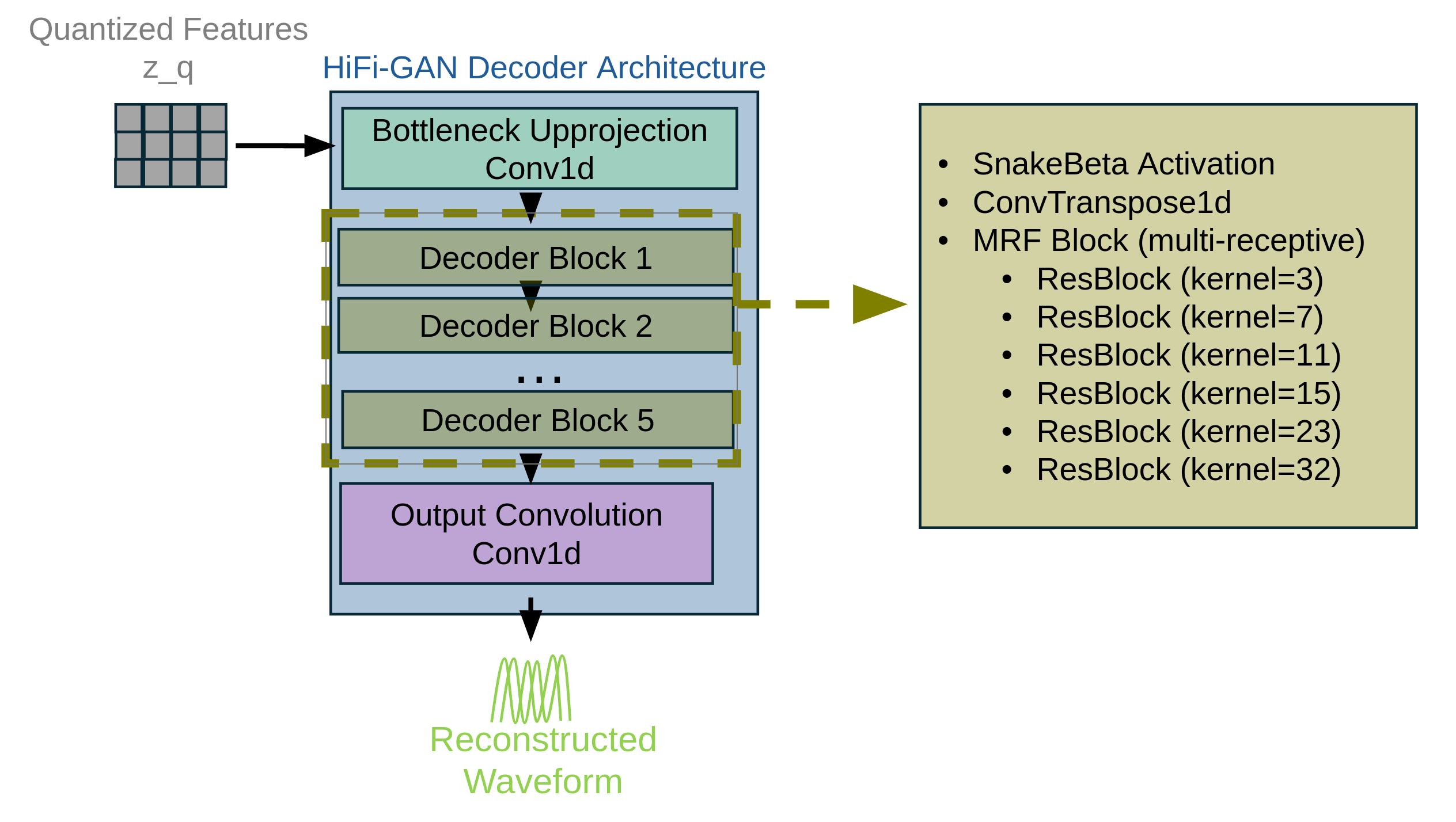
HiFi-GAN Decoder
The decoder upsamples quantized representations back to waveform. We use HiFi-GAN with DAAM gating in residual blocks
Decoder architecture:
The decoder upsamples quantized representations back to waveform through TransposeConv1D blocks with stride, progressing through channel dimensions: 512→384→256→128→64. Each block consists of upsampling followed by ResBlocks with DAAM gating (though disabled in current implementation). The total stride of 6×5×5×8×8 = 9600 matches the encoder, transforming the quantized input [B, 512, T_z] to output waveform [B, 1, T_wav].
ResBlock with DAAM:
Each residual block contains:
- Leaky ReLU activation
- Dilated convolution
- Residual connection
Decoder hyperparameters:
- Upsample kernels: [3, 7, 11, 15, 23, 32]
- Residual blocks: 8 per stage
Stage 2 Training Objective
Stage 2 optimizes the FSQ quantizer and HiFi-GAN decoder and the JEPA encoder.
Loss function:
\[\mathcal{L}_{\text{total}} = \mathcal{L}_{\text{rec}} + \lambda_{\text{stft}} \mathcal{L}_{\text{stft}} + \lambda_{\text{gan}} \mathcal{L}_{\text{gan}}\]1. Reconstruction Loss (L1):
\[\mathcal{L}_{\text{rec}} = \frac{1}{T_{\text{wav}}} \sum_{t=1}^{T_{\text{wav}}} |\hat{x}_t - x_t|\]where $\hat{x}$ is the reconstructed waveform and $x$ is the ground truth.
2. Multi-Resolution STFT Loss
For each STFT resolution $m$:
Spectral convergence: \(\mathcal{L}_{\text{sc}}^{(m)} = \frac{\| |S_m(\hat{x})| - |S_m(x)| \|_F}{\| |S_m(x)| \|_F}\)
Log-magnitude loss: \(\mathcal{L}_{\text{mag}}^{(m)} = \frac{1}{N_m} \| \log |S_m(\hat{x})| - \log |S_m(x)| \|_1\)
STFT configurations:
- FFT sizes: [2048, 1024, 512, 256, 128]
- Hop sizes: [512, 256, 128, 64, 32]
- Window: Hann
The MR-STFT loss uses L1 on magnitude and L1 on log-magnitude.
3. GAN Loss:
Multi-period discriminator (MPD) and multi-scale discriminator (MSD) provide adversarial feedback
Generator loss (least-squares GAN): \(\mathcal{L}_{\text{gen}} = \sum_{d \in \{MPD, MSD\}} \mathbb{E}[(D_d(\hat{x}) - 1)^2]\)
Feature matching loss: \(\mathcal{L}_{\text{feat}} = \sum_{d \in \{MPD, MSD\}} \sum_{l=1}^{L_d} \frac{1}{N_l} \| D_d^{(l)}(x) - D_d^{(l)}(\hat{x}) \|_1\)
Discriminator loss:
\[\mathcal{L}_{\text{disc}} = \sum_{d \in \{MPD, MSD\}} \left( \mathbb{E}[(D_d(x) - 1)^2] + \mathbb{E}[D_d(\hat{x})^2] \right)\]Training procedure:
The encoder parameters and decoder parameters receive the standard learning rate. A separate optimizer is used for the discriminators with half the generator learning rate. During each training step, the generator is updated with the combined reconstruction, STFT, and GAN losses. After a warmup period of 5000 steps, the discriminators are updated every step using detached reconstructions to prevent gradients flowing back to the generator.
Loss weights:
- $\lambda_{\text{stft}} = 2.0$
- $\lambda_{\text{gan}} = 0.1$
- Discriminator warmup: 5000 steps
- Discriminator update interval: 1 (every step after warmup)
Training hyperparameters:
- Optimizer: AdamW with $\beta_1 = 0.8$, $\beta_2 = 0.99$
- Learning rate: $1.5 \times 10^{-4}$ (decoder), $0.75 \times 10^{-4}$ (discriminator)
- Weight decay: $10^{-3}$
- Batch size: 8
- Training steps: 29,000
Experimental Setup
Dataset:
- LibriLight (large-scale unlabeled English speech corpus)
- Training split combined subset across the 2 stages: ~9,000 hours
- Validation split: separate held-out speakers
- Sample rate: 24 kHz
- Audio length: maximum of 15 seconds
Data preprocessing:
- Resample to 24 kHz if needed
- Convert to mono by averaging channels
- No other preprocessing (normalization handled by model)
Distributed training:
- GPUs: 2x NVIDIA A100 (80GB)
- Mixed precision: FP16 for forward/backward, FP32 for critical ops
- Gradient accumulation: 1 step
- Global batch size: 64 (Stage 1), 16 (Stage 2)
Inference:
During inference, the full pipeline operates as:
- Raw waveform → JEPA encoder → Latent features
- Latent features → FSQ quantization → Discrete tokens
- Discrete tokens → Dequantization → Quantized features
- Quantized features → HiFi-GAN decoder → Reconstructed waveform
Token rate: 47.5 tokens/sec (G=7 packing)
Model Architecture and Efficiency
| Component | Parameters | Notes |
|---|---|---|
| Stage 1: JEPA Encoder Training | ||
| Online Encoder | 121.7M | Trainable (context encoder) |
| Target Encoder (EMA) | 118.5M | (momentum update) |
| Predictor Network | 3.2M | Trainable (masked prediction) |
| Stage 1 Total | 240.2M | 121.7M trainable |
| Stage 2: Decoder Training | ||
| JEPA Encoder | 240.2M | Trainable via fine-tuning |
| FSQ Quantizer | ~0.01M | Trainable (finite scalar quantization) |
| HiFi-GAN Decoder | 69.2M | Trainable (waveform reconstruction) |
| Stage 2 Total | 309.5M | 69.3M trainable |
| Final Model (Inference) | ||
| Encoder only | 121.7M | Online encoder (no EMA needed) |
| FSQ + Decoder | 69.3M | |
| Inference Total | 191.0M | Compact single-pass model |
Training Efficiency
| Metric | Stage 1 (JEPA) | Stage 2 (Decoder) |
|---|---|---|
| Trainable Parameters | 121.7M (50.7%) | 69.3M (22.4%) |
| Training Steps | 24K | 29K |
| Batch Size | 32 | 8 |
| Learning Rate | 1.5e-4 | 1.5e-4 |
Key Efficiency Features:
- Two-stage training: Self-supervised pretraining (Stage 1) + supervised finetuning (Stage 2)
- Inference efficiency: 191M parameters (no EMA encoder needed at inference)
Evaluation Metrics
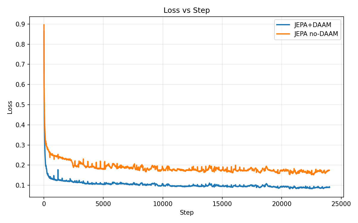
We employ qualitative evaluation metrics for our models, as all variants were trained with limited computational budgets and this work presents preliminary findings:
Baseline comparisons:
- JEPA baseline: JEPA encoder without DAAM gating
- WavLM-Large
: Pre-trained self-supervised model - JEPA with DAAM: JEPA encoder with DAAM gating
Audio Samples
Sample 1:
Original
Baseline JEPA
JEPA+DAAM
WavLM-Large
Sample 2:
Original
Baseline JEPA
JEPA+DAAM
Discussion
Why DAAM Improves JEPA Representations:
The integration of Density Adaptive Attention into the JEPA framework provides key advantages:
Comparison to Standard Attention Mechanisms:
Traditional softmax-based self-attention computes correlation between positions—”Which other timesteps are similar to this one?” producing pairwise similarity matrices.
DAAM computes statistical salience of features—”Which timesteps have unusual or informative statistical properties?” producing temporal importance weights based on Gaussian mixture modeling.
DAAM’s Gaussian framework can capture these patterns without requiring the quadratic complexity of full self-attention.
Limitations and Future Work
Current Limitations/Future work:
-
Fixed masking strategy: Block masking with fixed span lengths may not adapt to varying speech rates or linguistic structure. Future work could explore adaptive masking where span lengths depend on acoustic/linguistic boundaries.
-
Monolingual evaluation: Current experiments focus on English (LibriLight). Generalization to tonal languages, tone languages with lexical tone, and morphologically rich languages remains unexplored.
-
Models are trained on limited data: Current pre-training experiments have only been carried on a very small number of speech hours and conclusions are limited to emerging capabilities.
-
Cross-modal JEPA: Extend to audio-visual or audio-text joint embedding prediction for aligned multimodal representations.
Code Availability
The complete implementation of our JEPA+DAAM framework, including training scripts, model architectures, and data processing pipelines, is available in our public repository:
The repository includes:
- Stage 1 JEPA encoder training with DAAM
- Stage 2 decoder training with encoder
- FSQ quantization and mixed-radix packing algorithms
- HiFi-GAN decoder with optional DAAM gating
- DeepSpeed integration for distributed training
GitHub: https://github.com/gioannides/Density-Adaptive-JEPA
Conclusion
We introduced a two-stage self-supervised framework combining Joint-Embedding Predictive Architecture (JEPA) with Density Adaptive Attention Mechanisms (DAAM) for efficient speech representation learning. Stage 1 trains a JEPA encoder with DAAM-based gating to learn robust semantic representations via masked prediction using only MSE loss on masked regions. Stage 2 leverages these representations for reconstruction using L1 loss, multi-resolution STFT loss, and adversarial GAN losses with Finite Scalar Quantization (FSQ) and HiFi-GAN decoding.
Key methodological contributions:
-
DAAM-enhanced JEPA encoder: Gaussian mixture-based attention for adaptive feature selection during self-supervised learning
-
Efficient tokenization: Mixed-radix FSQ packing achieving 47.5 tokens/sec, nearly half the rate of existing neural audio codecs
-
Two-stage training: Pure self-supervised representation learning (Stage 1 MSE loss only) followed by reconstruction training (Stage 2 L1 + STFT + GAN losses)
The framework demonstrates how probabilistic attention mechanisms can improve representation learning (Stage 1) by dynamically identifying acoustically salient regions during masked prediction. This work establishes DAAM as a versatile component for speech processing architectures, with applications extending beyond codec design to any task requiring adaptive temporal feature selection.