Do Sparse Autoencoders (SAEs) transfer across base and finetuned language models?

TLDR (Executive Summary)

We explored whether Sparse Autoencoders (SAEs) can effectively transfer from base language models to their finetuned counterparts, focusing on two base models: Gemma-2b and Mistral-7B-V0.1 (we tested finetuned versions for coding and mathematics respectively)
In particular, we split our analysis into three steps:
1. We analysed the similarity (Cosine and Euclidian Distance) of the residual activations, which was highly correlated with the resulting transferability of the SAEs for the two models.
2. We computed several performance metrics (L0 Loss, Reconstruction CE Loss, Variance Explained) of the base SAEs on the fine-tuned models. Almost all metrics agreed on a significant degradation of the SAE performance for the Gemma-2b model, and remained within a reasonable range for the Mistral-7B model, indicating a much better transferability.
3. We took a further step by operationalizing the idea of transferability of SAE from base models to fine-tuned models by applying an approach from Towards Monosemanticity for studying feature universality through feature activation similarity and feature logit similarity. These similarity scores were mostly consistent with the results from the previous step, albeit with one caveat for the Gemma-2b model, suggesting that some SAE features may still transfer even if the overall SAE performance is poor for the finetuned model.
Overall, our results agree with previous work that studied Instruct models. That is, SAEs transferability seems to be model-dependent and sensitive to the finetuning process.
We make our code repository public to facilitate future work in this direction.

1. Introduction and motivation

1.1 What are SAEs and why do we care about them

We find ourselves in a world where we have machines that speak fluently dozens of languages, can do a wide variety of tasks like programming at a reasonable level, and we have no idea how they do it! This is a standard mechanistic interpretability (a.k.a. mech interp) pitch - a field that is trying to express neural networks’ behaviours as human-understandable algorithms, i.e. reverse engineer algorithms learned by a neural network (or a model, in short). The main motivation is that even though we know the exact form of computation being done by the model to transform the input (e.g. text prompt) to the output (e.g. text answer), we don’t know why this computation is doing what it’s doing, and this is a major concern from a standpoint of AI Safety. The model can perform the computation because it’s genuinely trained to perform the task well, or because it learned that doing the task well correlates with its other learned goals like gaining more power and resources. Without understanding the computation, we have no direct way of distinguishing between the two.

The solution proposed by mechanistic interpretability is closely analogous to reverse engineering ordinary computer programs from their compiled binaries. In both cases, we have an intrinsically non-interpretable model of computation - a sequence of binary instructions performed on a string of 0s and 1s, and the (mathematical) function of the neural network’s architecture applied with its learned parameters (weights)This is a pretty important analogy to understand and you can read more about it in [this Anthropic post](https://transformer-circuits.pub/2022/mech-interp-essay/index.html) where it's explained better. . Programmers know that a natural way to think about computer programs is mapping variables into other variables (or new states of existing variables), starting from some pre-initialized state. So, reverse engineering complied binaries boils down to (oversimplifying) identifying binary memory segments that correspond to variables, tracking how these segments change as the program is being executed, coming up with the explanations of the purpose of these variables, and ultimately arriving at the replication of the program source code - a sequence of human-understandable instructions.

But what makes us think that the same is possible for neural networks, especially the ones as large as the current Large Language Models (LLMs)? In particular, why should we even expect that neural networks solve tasks similarly to humans, and thus adopt the same “variable-centered” model of computation? While the proof-of-existence for the first question appeared relatively early (see Circuits thread by Chris Olah et al. for CNNs or a more recent work by Neel Nanda et al. for language models), the second question is a more general claim, and thus requires more general evidence. The first fundamental work that provided such evidence was the “Towards Monosemanticity” paper by Anthropic, which introduced Sparse Autoencoders (SAEs) for interpreting the language models’ activations. The activations are any intermediate state of the models’ computation, such as residual stream, MLP layers etc. and can be seen as analogous to a program’s memory state. And just as the program’s memory state can be decomposed into variables, the main purpose of SAEs is to decompose models’ activations into features.

A feature, in general, is a fuzzy term, and you can find some good attempts to define it here. For this post we’ll use the analogy with variables and link it to a very general definition of a feature as “a property of the input”. The link is pretty natural: the types and the number of variables a programmer needs to solve a task depends on the task itself (i.e. on the problem input). So for a model it would seem reasonable if it used different kinds of variables/features depending on its input: you don’t need a feature “this line is inside a for-loop in Python” in a poetry text, or a feature “this word rhymes with ‘sunset’” in the Python code. And given that models have a finite amount of parameters (which limits a total number of variables they can use), we should expect that they will utilize this kind of input-specificity to use as many unique features as they need to perform a specific task.

Why are sparse autoencoders called sparse? It’s actually deeply linked with the idea from the previous paragraph: if you want to use many features in a limited activation space (limited by a number of neurons), you have to exploit the fact that for any input, most of the features will not be there. So given that modern language models are trained to predict a next token in a huge variety of possible inputs, we should expect that any feature learned by the model will be sparse, i.e. it will be used by the model only for a small fraction of all possible inputs.

But wait, how is it even possible for a model to learn input-specific features if it has a low-dimensional activations space (where dimension equals the number of neurons) but a very high-dimensional input space? The answer is superposition - an idea of exploiting feature sparsity to store more features than dimensions in the activation space. It has a rich mathematical background and we invite an unfamiliar reader to learn more about it in the “Toy Models of Superposition” paper by Elhage et al.

Coming back to SAEs, they were introduced with all of these ideas in mind to solve superposition, i.e. to recover more than n features in an n-dimensional activation space of a model. How are they supposed to do it? The answer is once again in the name - autoencoders, which means that SAEs are neural networks with the “autoencoder” architecture, which is illustrated in a diagram below (borrowed from the great Adam Karvonen’s post):

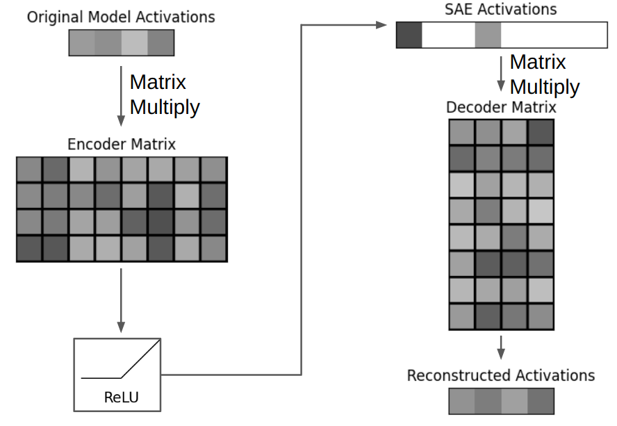
So the model activations are “encoded” into a high-dimensional vector of feature activations (top right, note that it always has many more elements than the model’s input), and this high-dimensional vector (a.k.a. “code”) is “decoded” back to reconstruct the input, hence the name “autoencoder”. We advise the reader to take a quick look at the “Towards monosematicity” appendix where this architecture is presented mathematicallyNote that it's different from the diagram in two ways: adding biases vectors **b** and using a transposed encoder/decoder matrix compared to what is seen in the diagram., but the core point to understand is that we’re interested in the right part of the above diagram: how the reconstructed activations are decomposed into a linear combination of feature vectors from the Decoder matrix (with the weights of a linear combination equal to SAE feature activations, due to how matrix-vector multiplication works). Mathematically, it means that for each input $x^j$ (which is the model’s activation vector at the place where we ‘attach’ the SAE - residual layer, hidden head activations etc.), we’re looking to express it in the following form:

\[\mathbf{x}^j \approx \mathbf{b} + \sum_i f_i(\mathbf{x}^j) \mathbf{d}_i\]

where $f_i(\mathbf{x}) = \text{ReLU}\left( \mathbf{W}_{enc} \mathbf{x} + \mathbf{b}_{enc} \right)_i$ are the feature activations that are computed in the left (“encoder”) part of the diagram, and $\mathbf{d}_i$ are the rows of the decoder matrix (or columns, if you take the transpose and multiply from the other side). Note that the diagram omits bias vectors $\mathbf{b}$ for simplicity, but conceptually they don’t change much: instead of decomposing the activation space, we’re decomposing a translation of that space by a fixed vector (because this is just easier for an SAE to learn).

If you think about it, it’s exactly what we hoped to do in an analogy with decomposing program memory into variable names! The variables are now features - vectors (directions) in the activation space. And if the autoencoder is doing a good job at reconstructing the input, we can expect that this decomposition (and hence the features) to make sense!

The last part is tricky though. Unlike variables that are deliberately used by humans to write sensible algorithms, there is no reason to expect that the features we recover with an SAE will be interpretable in a sense that a human can understand on which inputs they activate and can predict their “roles” based on that (e.g. which tokens they help to predict). But this is where the sparsity condition comes in: we don’t only want an SAE to reconstruct the input from a high-dimensional feature-activation representation, but we also want this representation to be sparse, i.e. have only a handful of non-zero feature activations at a time. We already touched on the reason for this - the hope is that we’ll be able to recover the “true” features used by the model in this wayIt's quite a slippery area to consider the logical relationship between the feature quality of being "truly used" by the model (analogously to correctly recovered variables from the compiled binary) and its interpretability. If the model came up with some genius way to solve a particular task using features no human can comprehend, would they still be considered as interpretable? The answer can vary from "no" to "kind of yes", because it can be argued that humans with their evolutionally developed problem-solving skills can eventually understand (i.e. interpret) how things work, even though it may not be obvious at a first glance. It's also discussed by Neel Nanda [here](https://dynalist.io/d/n2ZWtnoYHrU1s4vnFSAQ519J#z=dzkF4Sh89hg1GUJj5h2TiGVx) . And the way this is achieved is by imposing an L1-loss penalty on the feature activation vector, which intuitively incentivizes the model to not learn any features unless they are really useful in reconstructing the inputThere's also a better justified mathematical reason for sparsity, greatly explained [here](http://ufldl.stanford.edu/tutorial/unsupervised/SparseCoding/). Essentially, by learning to decompose the model's activation space into feature activations, we're trying to find an overcomplete basis of feature directions (a basis with more than n vectors in an n-dimensional space), which is impossible to do without imposing some additional criteria. The ["Toy Models of Superposition"](https://transformer-circuits.pub/2022/toy_model/index.html) is also incredibly helpful to refine one's intuition about this. .

1.1.1 SAE features for AI Safety

The traditional view in mech interp has been that one cannot interpret the model’s weights if one cannot interpret the neurons that the weights are connecting. But due to the neurons polysemanticity (a consequence of superposition), interpreting individual neurons in the language model is extremely hard if at all possible. That’s where SAEs come to the rescue: by revealing the directions in the neuron activation space (i.e. features) that have a clear, interpretable meaning, they allow for a new form of circuits analysis: instead of interpreting weights between neurons, we can instead interpret weights connecting features. Thus the SAE features potentially serve as a new “basis” for circuit analysis, and some of the recent work e.g. by Marks et al. and Batson et al. has already started exploring this idea and producing the first results.

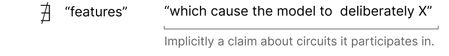
So what does this mean for AI Safety? We’ll cite the Anthropic team’s view on this topic (layed out in their “Interpretability Dreams” post and in the “Strategic Picture” section of the Toy Models paper):

We’d like a way to have confidence that models will never do certain behaviors such as “deliberately deceive” or “manipulate.” Today, it’s unclear how one might show this, but we believe a promising tool would be the ability to identify and enumerate over all features.

Ultimately we want to say that a model doesn’t implement some class of behaviors. Enumerating over all features makes it easy to say a feature doesn’t exist (e.g. “there is no ‘deceptive behavior’ feature”) but that isn’t quite what we want. We expect models that need to represent the world to represent unsavory behaviors. But it may be possible to build more subtle claims such as “all ‘deceptive behavior’ features do not participate in circuits X, Y and Z.”

Summarizing, the hope is to be able to prove statements of the following form:

1.2 Finetuning models is a challenge to AI safety - SAEs to the rescue?

After outlining the procedure behind SAE-interpretability, we can answer a more general question: why is it relevant to translate the matrix language of neural networks (not more understandable to us than binary code) into a human-readable algorithmic language? There are several reasons, but, among the others, once we are able to do so, we can understand what features of an input a model identifies before predicting an answer. This can allow us to identify when a model is learning to deploy features spuriously correlated with the actual labels (an intuitive example here) or when the model is even lying to us. In both of these cases, it is a primary safety concern that these behaviors are not occurring in our model when used in production. Moreover, SAE-interpretability allows us to gain some insight into solving these problems precisely!

Nevertheless, reality is often rougher than abstraction, and mechanistic interpretability suffers from one big problem: once we crack the interpretation of a model, we are only able to decode what is going on inside a singular, particular model, and not all models with the same architecture and different weights. Luckily, to have a model that shows emergent abilities, we need a lot of compute, which remarkably restricts the Pareto frontier of competitive models and therefore the number of pre-trained models that we need to interpret. Therefore, one could think that if we manage to get some good SAE-interpreters for these few, we will be done. This may not be true! While indeed there are few state-of-the-art models, there are tons of finetuned versions of them (hugging face reached 1 million of models), which are quite cheap to obtain compared to pretraining. If a simple finetuning will make the model uninterpretable, then we might be in danger. This could be the case, as previous studies showed that alignment can be erased with a small finetuning. Then we ask ourselves:

Is the interpretability of a model as weak as alignment to finetuning?

In this post, we try to answer these questions and extend the positive results derived from a similar study by Kissane et al., where SAEs for the residual stream have been shown to be easily transferable (at the cost of some finetuning).

Lastly, we want to remark how this kind of study derives its importance from the weakness of outer alignment forced by some ad-hoc finetuning. Indeed, if interpretability is more resistant to being broken than alignment, the path towards AI safety could be reached via digital neuroscience, rather than simply through external finetuning.

2. Problem setup

In choosing finetuned models to work with, we tried to strike a balance between the potential relevance of these models (how many people will actually use similar models), and the availability of pre-trained SAEs from the SAELens library we used. So, we arrived at the following models and their finetunes:

Gemma-2b (v1) -> Gemma-2b-it-finetuned-python-codes finetune on Python code by Dishank Shah.
Mistral-7B (v0.1) -> MetaMath-Mistral-7B finetune on math problems by Meta from their MetaMath paper by Yu et al.

We then loaded the following SAEs for these models from SAELens (SAE layer numbering starts from 0):

Model	SAE Release	SAE Layer	N Features
Gemma-2b (v1)	gemma-2b-res-jb by Joseph Bloom	Residual layer #6	16384
Mistral-7B (v0.1)	mistral-7b-res-wg by Josh Engels	Residual layer #8	65536

Two important things to note:

Gemma-2b SAE was trained on the base Gemma-2b model, while our Gemma-2b finetune was obtained from the instruct model, so there was one more “finetuning step” compared to the Mistral-7B case.
Both finetunes that we used are full finetunes (with respect to the base model), i.e. no layer was frozen during the finetuning process. This is important for our SAE study, because all SAEs would trivially generalize (in terms of their reconstruction quality) if they were applied at the layer where activations are not affected a priori by the finetuning process.

2.1 Studying “default” transferability

Similarly to what Kissane et al. did with the instruct models, we’ll study the SAE transferability “by default”. That is, we’ll take an SAE trained on the base model, and apply it to the finetuned model to see if it maintains its performance (operationalized below). We won’t do any additional finetuning of our SAEs (on the activations from the finetune model), but as the same results from Kissane et al. indicate: even when SAEs do not transfer by default, they can be finetuned relatively cheaply to recover their performance.

Prior to evaluating the SAEs’ performance, we computed different similarity metrics for residual stream activations at the specific layer our SAEs are used for. The goal was to obtain some sort of a prior probability that our SAEs will transfer to the finetune model: the more similar the activations are, the higher is the (expected) probability that our SAEs will transfer. On the one hand, this analysis can be used as a first step to select a fine-tuned model from the thousands available on Hugging-Face. On the other hand, further studies can try to analyze whether the phenomenon of SAE transferability actually correlates with the difference between activations of the base and fine-tuned models (which we treat here only as an unproven heuristic).

2.2 Evaluating SAEs performance

Designing rigorous approaches to evaluate the SAEs’ performance is an open problem in mechanistic interpretability. The main complicating factor is that we’re interested not so much in the SAEs reconstructed output, but rather in the SAE feature activations and feature vectors. However, measuring whether the SAEs features are interpretable or whether the features “are truly used by the model” is not straightforward. For our work, we’ll just start with computing standard evaluation metrics proposed either in the original “Towards monosemanticity” paper, or used in the later work, e.g. this one by Joseph Bloom:

L0 loss, namely the number of non-zero values in the feature activations vector. If the features retain their sparsity, we should expect L0 loss to be low compared to the total number of features, with the fraction being usually less than 1% ($\frac{L_0}{N_{\text{features}}} < 0.01$)
Reconstruction Cross-Entropy (CE) loss (a.k.a. substitution loss) which is computed as follows:
1. Run the model up to the layer where we apply the SAE, get this layer’s activations
2. Run the activations through the SAEs, obtaining the reconstructions
3. Substitute the original activations with the reconstructed activations, continue the forward pass of the model, and get the corresponding cross-entropy loss
Variance explained, is one of the standard ways to measure the difference of original activations and the activations reconstructed by the SAE. Specifically, we’ll use $R^2$ score a.k.a. Coefficient of determination
Feature density histograms: as explained by Joseph Bloom, ideally the features should be “within good sparsity range”: not too sparse (e.g. when the features are “dead” and never activate) and not too dense (e.g. activating in more than 10% of the inputs). In both edge cases, anecdotally the features are mostly uninterpretable. One (rather qualitative) way to check this is to plot feature histograms:
1. Run a given sample of tokens through the model, and get the SAE feature activations.
2. For each feature, record the number of times (tokens) it had a non-zero activation.
3. Divide by the total number of tokens to get the fraction, and take the log10 of it (adding some epsilon value to avoid log-of-zero)
4. Plot the histogram of the resulting log-10 fractions (the number of histogram samples equals to the number of features)

We’ll compute these metrics first for the base model and its SAE to get a baseline, then for the finetuned model with the same SAE, and compare the resulting metrics against the baselineEven though density histograms are not technically a metric, we can infer quantitative metrics from them like the number of dead features. The dataset used in both cases is the original training dataset of the corresponding SAE:

Fineweb dataset for Gemma-2b.
The Pile dataset for Mistral-7B.

Based on the feature density histograms, we additionally zoomed in on individual features to see how well they transfer using feature activation similarity and logit weight similarity, as elaborated in the later section of this post.

3. How similar are residual activations of finetuned models?

Before analyzing the SAE metrics on the finetuned models, we will visualize some easier computations on the residual activations (at the residual stream of the layer where we apply the corresponding SAE) to get a sense of the SAE transferability. Specifically, we are interested in the similarities between the base and finetuned model activations. We consider two metrics: the Cosine Similarity and the Euclidian Distance, for the model and datasets specified above with the Gemma-2b Python-codes and Mistral-7b MetaMath finetunes respectively.

Computing the Cosine Similarities and Euclidian Distances of the activations yields a tensor of shape [N_BATCH, N_CONTEXT] (each token position is determined by its batch number and position in the context). A simple metric to start with is to consider the global mean of the Cosine Similarities of the activations across both batch and context dimensions, giving a single scalar representing the overall similarity. This can be seen in the following table:

Model/Finetune	Global Mean (Cosine) Similarity
Gemma-2b/Gemma-2b-Python-codes	0.6691
Mistral-7b/Mistral-7b-MetaMath	0.9648

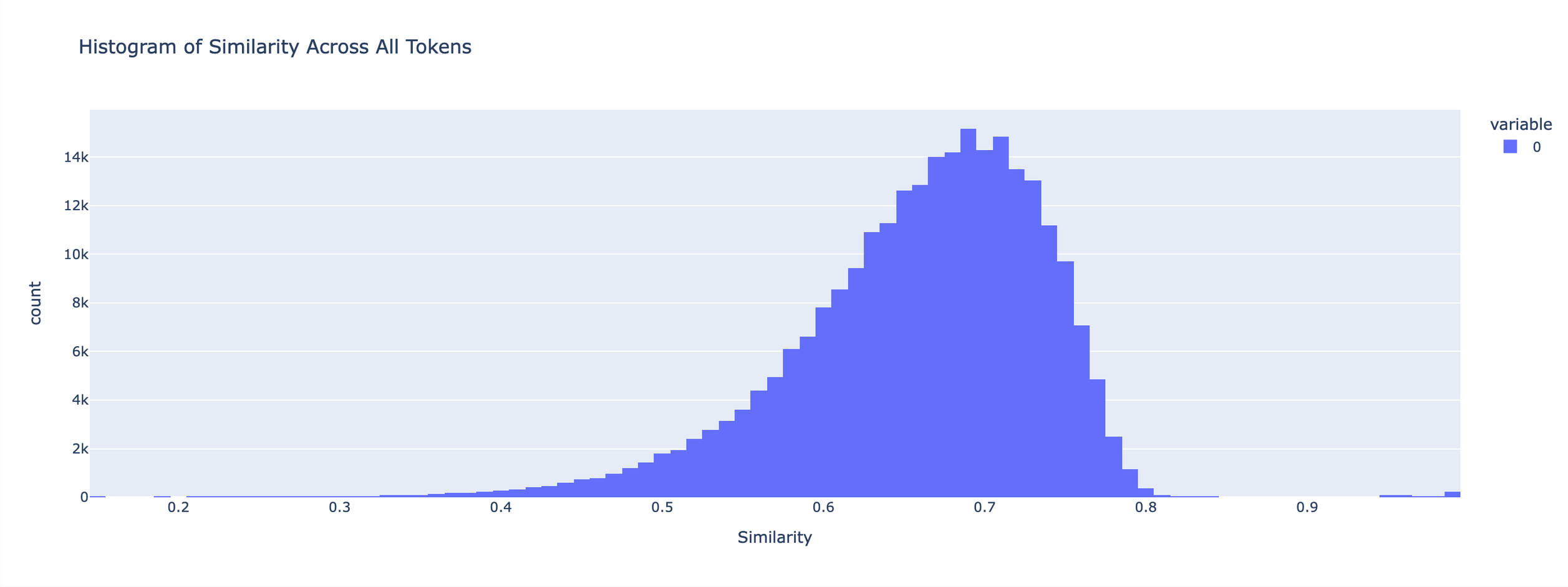
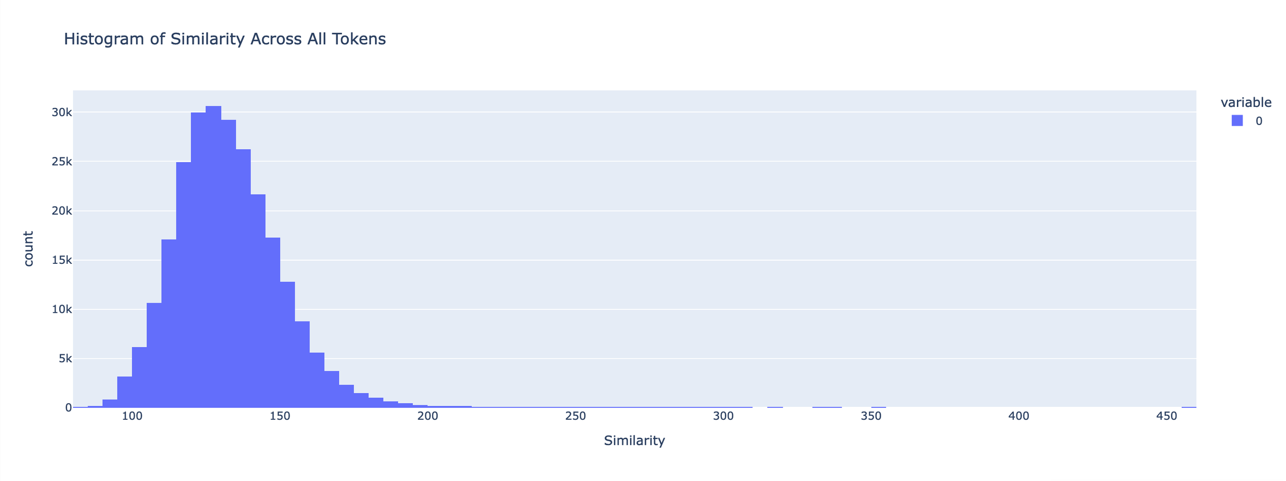
This already suggests much better transferability of the Mistral-7b SAE for its MetaMath finetune. For a more fine-grained comparison, we flatten the similarities into a N_BATCH * N_CONTEXT vector and plot the histogram across all tokens:

Gemma-2b - Cosine Similarity Histogram

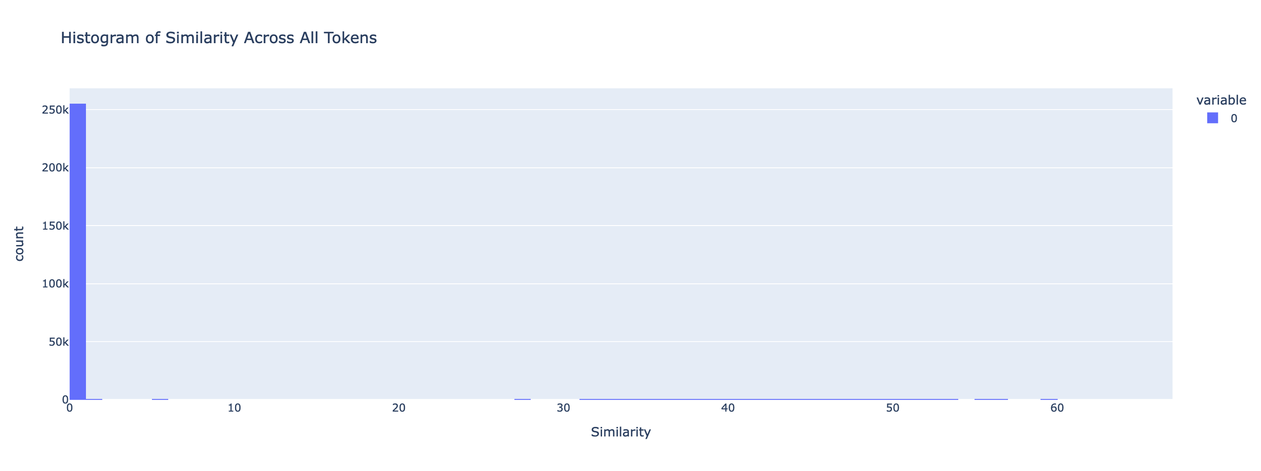
Mistral-7b - Cosine Similarity Histogram

Gemma-2b - Euclidian Distance Histogram

Mistral-7b - Euclidian Distance Histogram

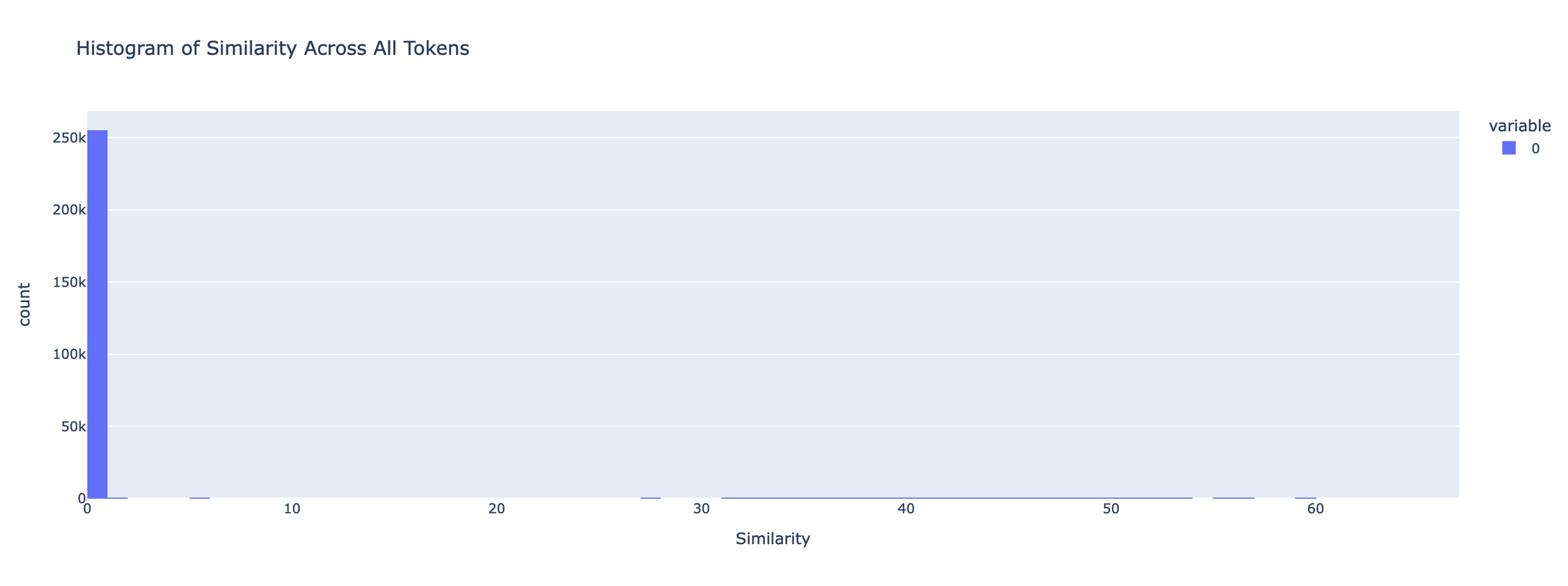
We can see how the Cosine Similarities for Mistral-7b are concentrated around a value close to 1, whereas the Gemma-2b similarities are more spread around the mean of 0.66 (higher variance). The Euclidian Distances histogram shows a similar distinction, with the Gemma-2b distances being spread around a mean of around 120, while the bulk of Mistral-7b distances stay at a low value.

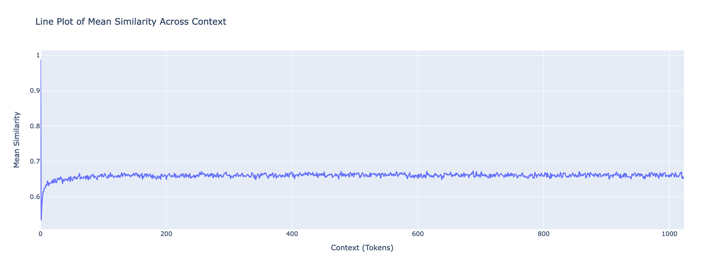
We also visualize the per-context mean of Cosine Similarities and Euclidian Distances. We compute the mean across batches but preserve the context dimension, giving a tensor of shape [N_CONTEXT], which reflects how similarity changes over the context length.

Gemma-2b - Cosine Similarity Context Line

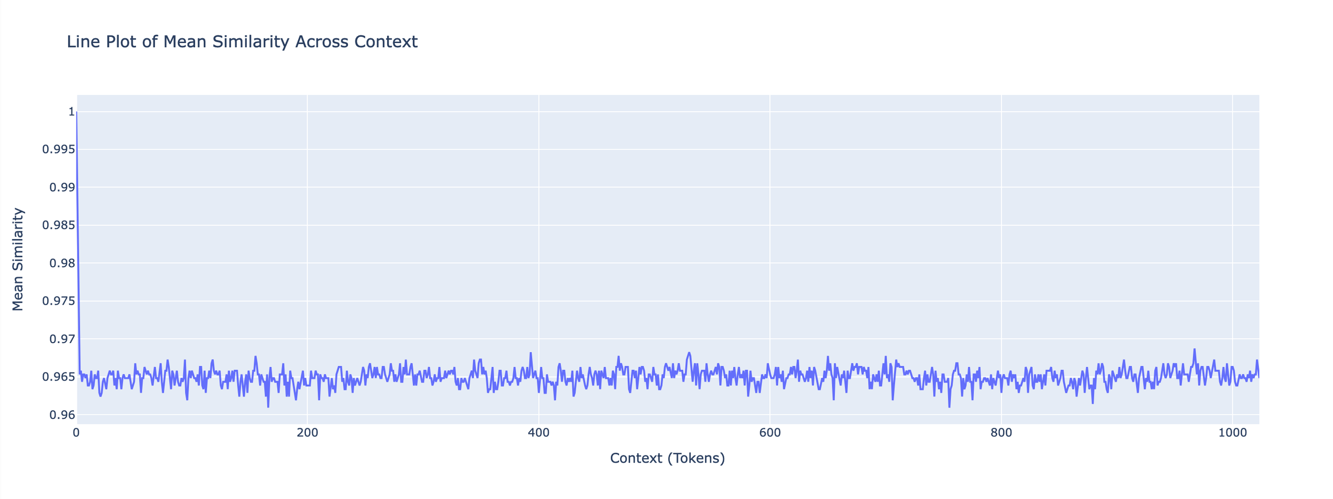
Mistral-7b - Cosine Similarity Context Line

Gemma-2b - Euclidian Distance Context Line

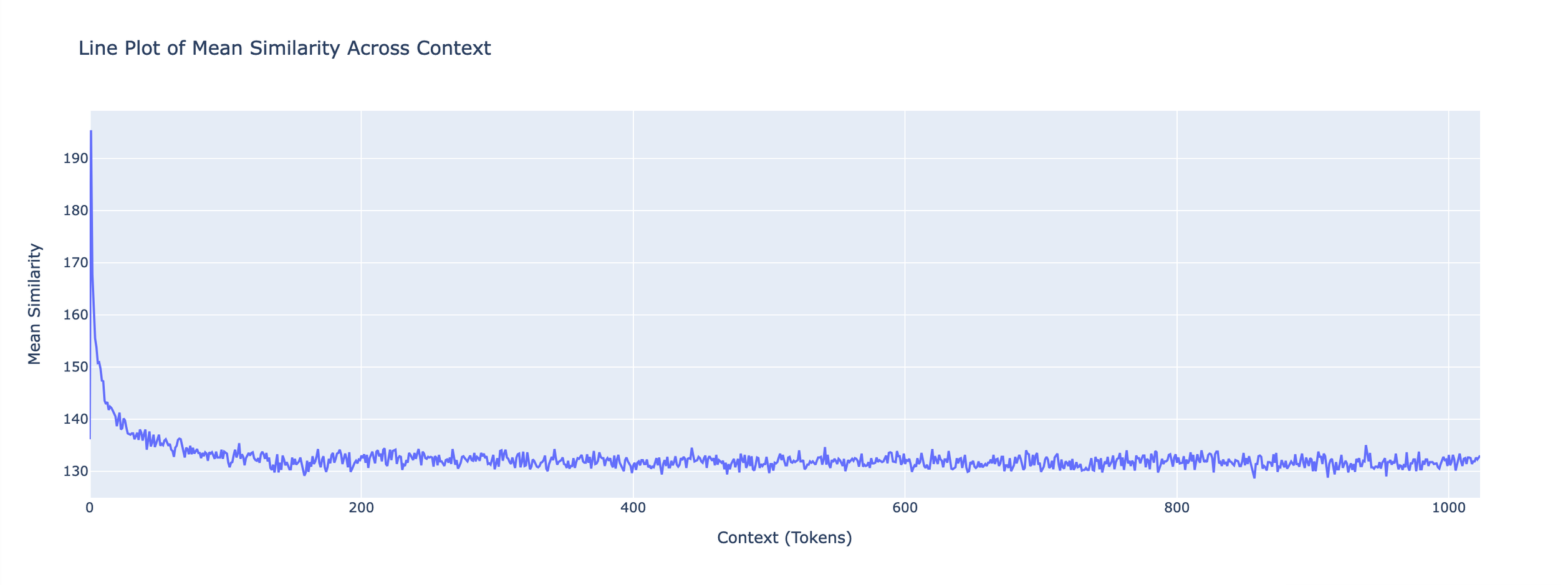
Mistral-7b - Euclidian Distance Context Line

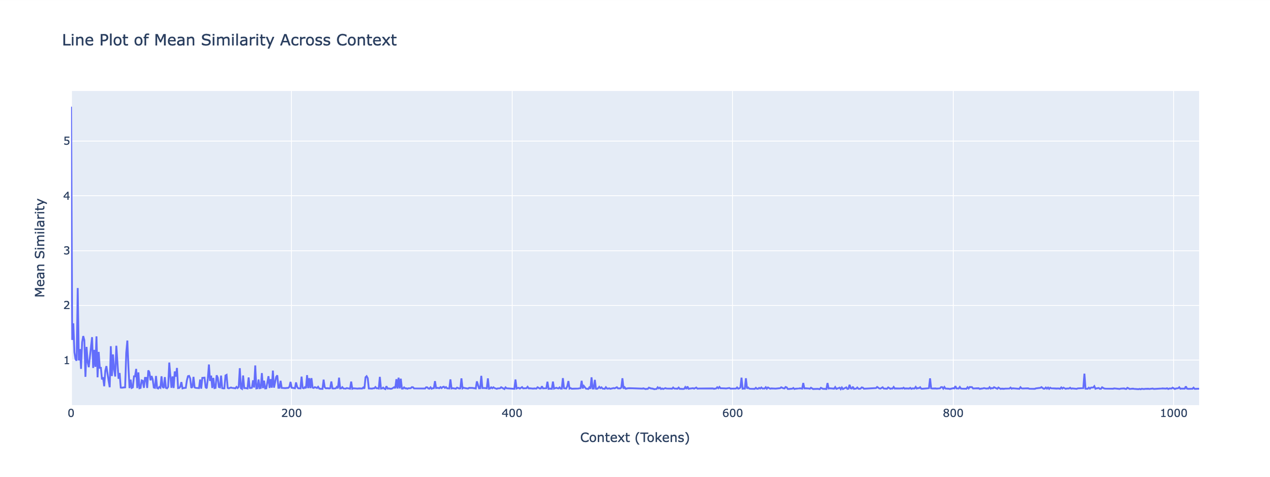
In the above, we can see how the similarities and distances stabilise quickly after a few tokens of context, albeit around different values. Both models start with close to 1 similarity for the first token, and then stabilize after a few tokens.

These results already anticipate a considerable difference in the transferability of the SAEs for the two models, which will be explored more in-depth in the following section.

4. How well do the base SAEs work on the finetuned models?

4.1 Methodology

In this section, we’ll compute a set of standard SAE metrics for base and finetuned models, using the same base SAE in both scenarios (i.e., the SAE that was trained on the base model activations):

For the base model:
1. we sample input tokens from the original SAE training dataset
2. pass the tokens through the base model to get the model’s activations
3. pass the activations through the SAE to get the feature activations
4. complete the forward pass of the base model to get the final loss (used afterward for the reconstructed loss)
Then we repeat the same steps for the finetuned model, using the same tokens dataset
Finally, we compute the metrics mentioned in the Evaluating SAEs performance section.

4.2 Technical Details

Before delving deeper into the results, we want to point out three technical details:

The sample size used across nearly all experiments is 256K tokens
Similarly to Kissane et al. we observed a major numerical instability when computing our reconstruction loss and variance explained metrics. As the authors noted:

SAEs fail to reconstruct activations from the opposite model that have outlier norms (e.g. BOS tokens). These account for less than 1% of the total activations, but cause cascading errors, so we need to filter these out in much of our analysis.
To solve this problem we used a similar outlier filtering technique, where an outlier is defined as an activation vector whose (L2) norm exceeds a given threshold. We tried several ways to find a “good” threshold and arrived at values similar to those used by Kissane et al:
- 290 norm value for the Gemma-2b model
- 200 norm value for the Mistral-7B model
Using these threshold values, we found that only 0.24% activations are classified as outliers in the Gemma-2b model, and 0.7% in the Mistral-7B, agreeing with the Kissane et al. result that these outliers account for less than 1% of activations. It should be noticed, however, that we only used this outlier filtering technique for our reconstruction loss & variance explained experiments to avoid numerical errors. In practice, it means that for this experiment the true sample size was a little smaller than for the other experiments, equal to $\left( 1 - \text{outlier_fraction} \right) \times 256{,}000$ with the $\text{outlier_fraction}$ defined above.

4.3 Results

In the following table, we report the results for the first experiment with the Mistral model pair:

Model\\Metric	L0 Loss	Clean CE Loss	Reconstruction CE Loss	Loss Delta	$$R^2$$ Score (Variance Explained)	Dead Features (%)
Mistral-7B	83.37	1.78	1.93	0.15	0.68	0.76%
Mistral-7B MetaMath	90.22	1.94	2.1	0.16	0.58	0.64%

As you can see, the L0-Loss of the features and variance explained increase a bit, but the reconstruction loss delta is almost the same! It suggests that our Mistral SAE may still transfer after finetuning, although with a slightly worse reconstruction quality. Let’s compare these results with the Gemma-2b and its Python finetune:

Model\\Metric	L0 Loss	Clean CE Loss	Reconstruction CE Loss	Loss Delta	$$R^2$$ Score (Variance Explained)	Dead Features (%)
Gemma-2b Base	53.59	2.65	3.16	0.51	0.97	48.1%
Gemma-2b Python-codes	84.74	3.29	7.5	4.21	-10.27	0.1%

Now, this is what bad SAE transferability looks like! But actually this should come as no surprise after the Kissane et al. result: they concluded that Gemma-2b SAEs do not transfer even between the base and the instruct models, so when you add an additional finetuning step on top of the instruct, it’s completely expected that the metrics will get even worse. The authors explain this behavior with an abnormal weights deviation in the instruct model:

Here we show that the weights for Gemma v1 2B base vs chat models are unusually different, explaining this phenomenon (credit to Tom Lieberum for finding and sharing this result):

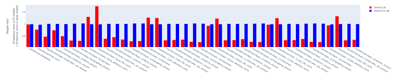
But what effect does this have on the SAE features? Well, we could expect that if an SAE is no longer able to reconstruct the input activations, it will always “hallucinate” - any features it “detects” will not make any sense. Let’s see if this expectation holds in practice for the Gemma-2b model.

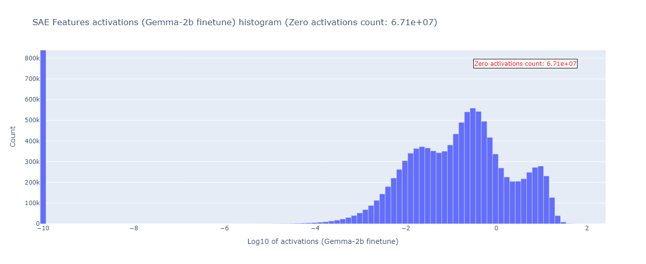
We’ll start with the feature activations histogram plot. In general, this kind of histogram gives little insight since you will always have a large mode at 0 due to feature sparsity, and some kind of log-normal distribution at non-zero activations. Indeed, this is what happens in the base Gemma-2b model, when we plot its log10 feature activations histogram:

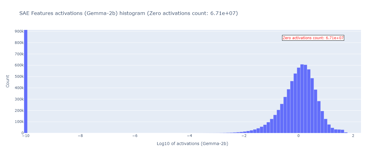
Two things to note:

The first bar’s count value is clipped - it’s much larger than 900k, equal to more than 6 million.
We used a smaller sample size for this experiment due to the need to store all the feature activations in memory to plot the histogram - here the sample size is equal to 128K.

With this in mind, let’s compare it with the same kind of histogram for our Gemma-2b finetune (where the features are given by the same SAE):

If that’s not a characterization for “cursed”, we don’t know what is! Instead of a nice bell curve, we now have some sort of a 3-mode monster in the non-zero activations section. To be clear - nothing like that was present when we repeated this experiment for the Mistral-7B: we obtained the well-expected bell curves with similar mean and standard deviation for both base and finetuned models. We don’t have a good explanation for this Gemma-2b anomaly, but we’ll try to give some deeper insight into what happens with the SAE features in the next section.

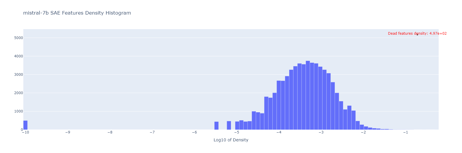
Let’s move on to the feature densities plot, which was produced as described in the Evaluating SAEs Performance section. Starting from Gemma-2b:

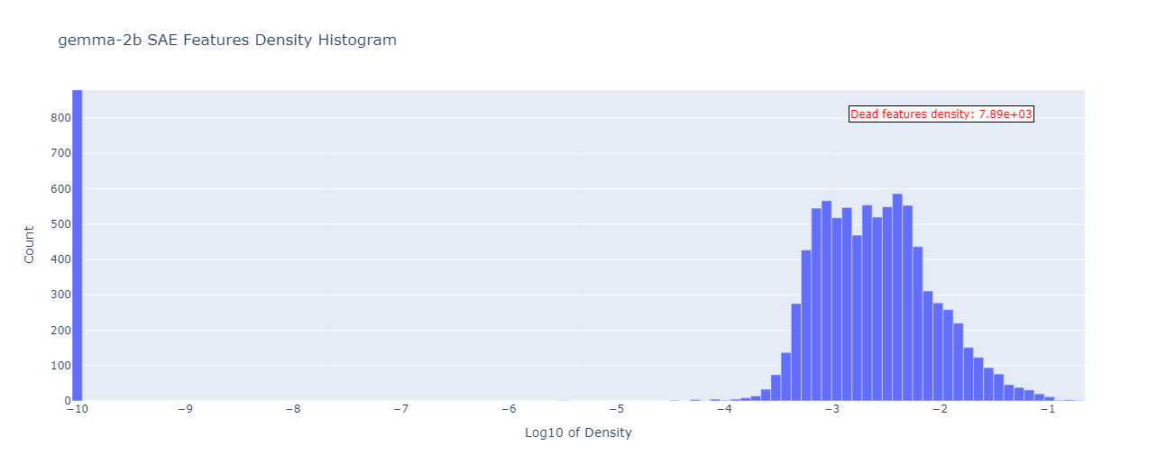
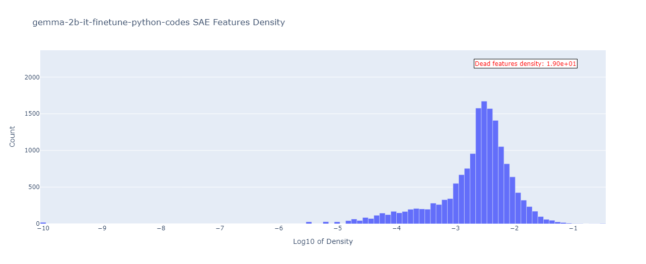
As expected from the above results, the two plots have little in common. We see that most of our dead features (in the base model) turn alive in the finetuned one! To see where exactly these dead feature densities land in the finetuned model (what are their new densities), we also made a parallel coordinate plot (below we show two versions of the same plot: with different density ranges highlighted):

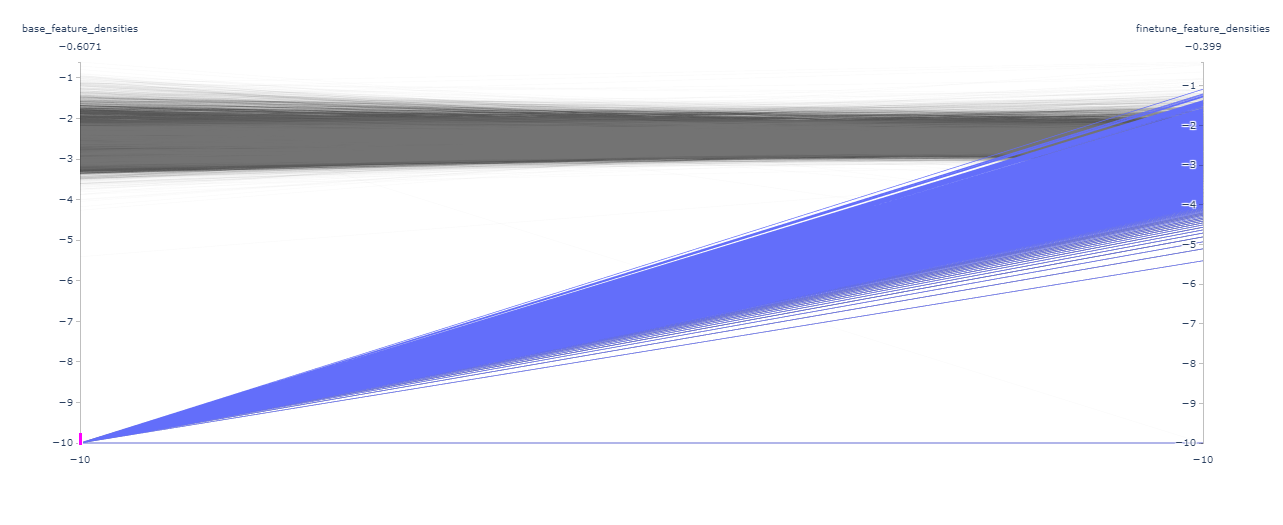
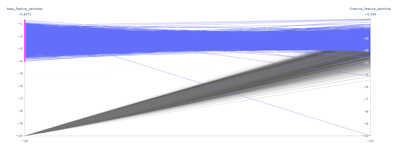
So it looks like the dead features spread out quite widely in the finetuned model, contributing to more probability mass before the -3 log-density. As for the dense features (-4 to -1 log density) in the base model, their density interval gets squeezed to (-3, -1) in the finetuned model, causing a sharp mode near the -2.5 log-density value.

We’ll continue the Gemma-2b investigation in the next chapter, and conclude this section with the Mistral-7B feature density histograms:

We can see that for Mistral the feature densities distribution almost doesn’t change after the model finetuning! The only slight difference is in the number of dead features: the finetuned Mistral has around 80 dead features less than the base one. To zoom in closer, we also show the parallel coordinate plot:

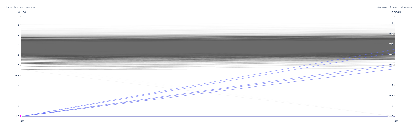
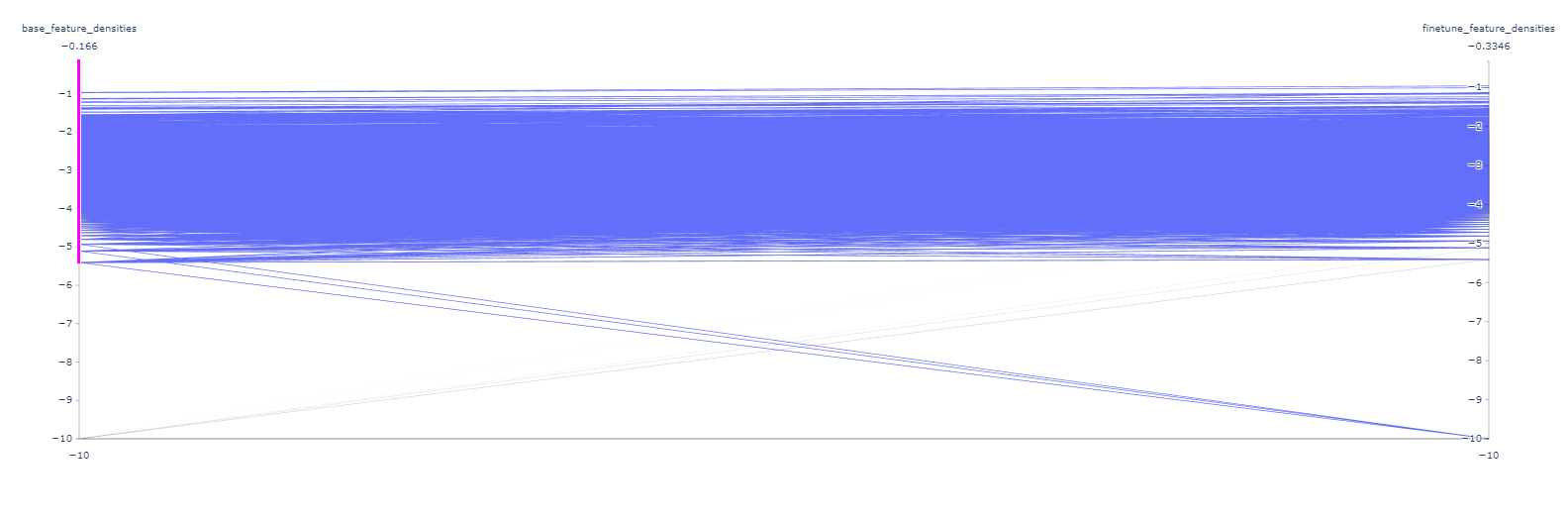
So yes, a small number of features do turn alive, but also some features (even a smaller amount) turn dead in the finetuned model! Overall though, the feature densities look very similar, with the Pearson correlation of their log10 densities equal to 0.94 (versus 0.47 for the Gemma-2b case).

5. Do the base SAE features transfer to the finetuned model?

We want to motivate this section with a more thoughtful consideration of the question what is the best way to operationalize SAE transferability. In the previous section, we simply checked the standard SAE evaluation metrics to see how well they reconstruct the activations. But this doesn’t necessarily reflect the main goal of using SAEs - interpreting the model.

As noted in the SAE features for AI Safety section of our post, the end goal of using SAEs for interpretability is to be able to use features as the basis for circuit analysis. And if we assume that some kind of circuit analysis has been done for the base model to prove that it doesn’t implement certain undesirable behaviors, the most ambitious operationalization of SAE transferability (for AI Safety) would be the ability to apply the same kind of circuit analysis with the same SAE (or the finetuned one) to prove or disprove that the finetuned model is safe.

In our case of studying transferability “by default”, the better way to demonstrate it is to show that our SAE features “stay relevant” in the finetuned model, so that we can expect that they still potentially serve as the basis for circuit analysis. Showing this rigorously would be a really difficult task (partly because there’s no standard way to do circuit analysis in the SAE basis yet) and it’s out of scope for this blog post. What we did instead is apply an approach from Towards Monosemanticity for studying features universality:

Normally to study if a feature from model A is conceptually the same (has the same “role” in the model) as another feature in the model B, one can compute
- feature activation similarity: represent a feature as a vector of its activations across a given sample of tokens, obtaining a feature activations vector → do it for model A’s feature, model B’s feature and compute a correlation between their activations vectors.
- feature logits similarity: represent a feature as a vector of its logit weights (for each token of the vocab a logit weight is the relative probability of that token as predicted by the feature direct effect), obtaining a feature logit vector→ do it for model A’s feature, model B’s feature and compute a correlation between their logit vectors.
So, we call model A our base model, model B - the corresponding finetune, and compute feature activation similarity and logits similarity for a given sample of the SAE features (which are the same for the base and finetuned models).

This can be seen as a (very) rough proxy for “the feature is doing the same job in the finetuned model”, and we call it the “feature transferability test”.

5.1 Feature Selection Procedures

Conceptually, dead features are completely different from the ordinary features: as explained by Joseph Bloom, they represent permanently lost capacity in an SAE and thus are merely an artifact of the SAE trainingEssentially, an SAE is saying “If I cannot find relevant features for reconstructing my input anymore, I’m going to learn a direction(s) in the activation space that is orthogonal to all the inputs I’ve seen, so that I get zero activations for the features I cannot learn and thus I’m no longer penalized by sparsity, at least”. If a feature was dead in the base model but is no longer dead in the finetuned one, it implies a distributional shift in the activation space (for which the SAE was not adapted, but could potentially be adapted by finetuning). So we decided to make a separate analysis of dead features and “regular” features, that we defined as features with a log10 density between -5 and -1.

By dead features, we mean features that are exclusively dead (never activating across our entire 256K sample of tokens), i.e. dead only in one of the models:

a “dead base” feature is a feature that is dead in the base model, but not in the finetuned one
a “dead finetune” feature is a feature that is dead in the finetuned model, but not in the base one.

We observe that only a handful of features are dead in both models, so we think our definitions give more information on what we’re analysing.

Then, our approach for the rest of this section looks as follows:

We sample max 100 exclusively dead features and 1000 regular features using our density histogram values for each base model and its finetune.
We convert these features to their activation vector and logit vector representations for both the base model and its finetune.
For each regular feature, we compute their activation similarity and the logits similarity with respect to the corresponding finetune, and for the exclusively dead features - their activation error:
- We cannot really compute the activation similarity as a correlation score if one of the feature’s activation vectors is constantly 0, i.e. the feature is dead. In this case we take the log10 of these activation vectors (with 1e-10 as the epsilon value to avoid a log of zero), take the Mean Absolute Error of the resulting vectors and call it activation errorIt makes little sense to compute dead features logit similarity: if the feature never activates, it doesn’t matter what its logit effect is - it will never manifest itself in the model. .
Additionally, we plot a histogram of similarities for each feature type, since we observed a significant deviation of the similarity score (mainly activation similarity) in some experiments.

5.2 Gemma-2b features transferability test

One could say that in the Gemma-2b case, it’s obvious from the previous results that our SAE doesn’t transfer. But we could imagine a case where some (perhaps a tiny fraction) of our SAE features from the regular density interval do still transfer, so we decided to conduct this experiment anyway.

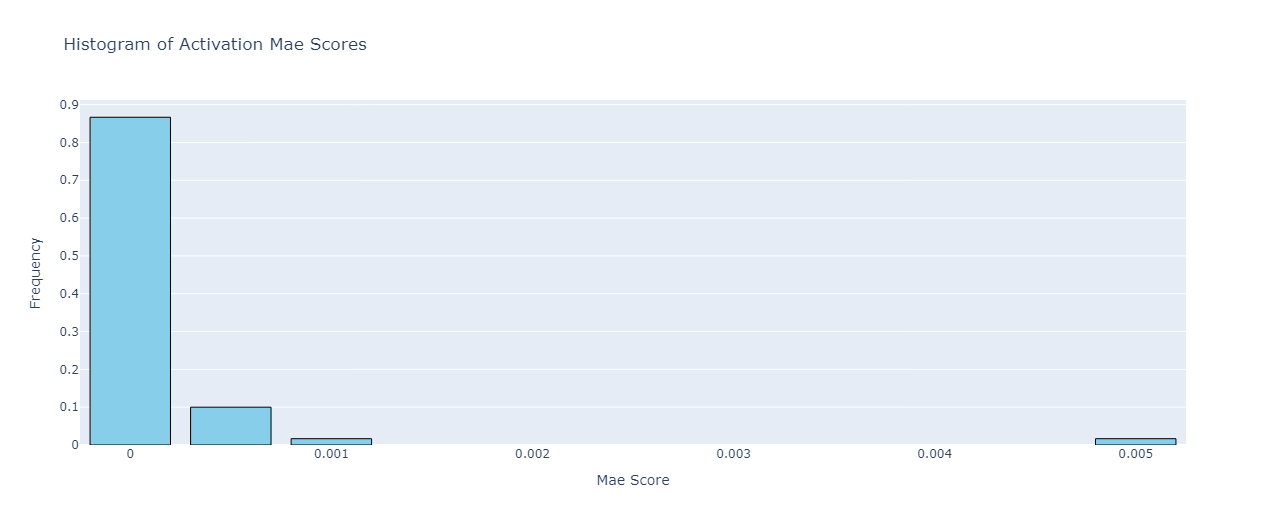
Starting with the features that are exclusively dead in the base model, their mean activation error for Gemma-2b and Gemma-2b python-codes finetune is 0.025. A histogram of these 100 activation errors is given below:

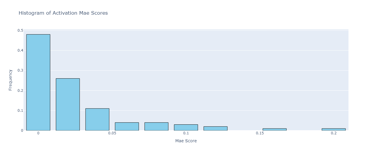
This made us think that “dead features turning alive” anomaly is not so much of an anomaly, because the dead features activate only (very) slightly in the finetuned model. The max activation value across all 100 dead features in the finetuned model was 1.1, indicating that our “dead feature direction” is only slightly off in the finetuned model, and can be easily adjusted by SAE finetuning.

As for the features that are exclusively dead in the finetune model, Gemma-2b had only two of them on our sample, with the activation error equal to 0.34 and 3.19, which is considerably higher than in the previous case.

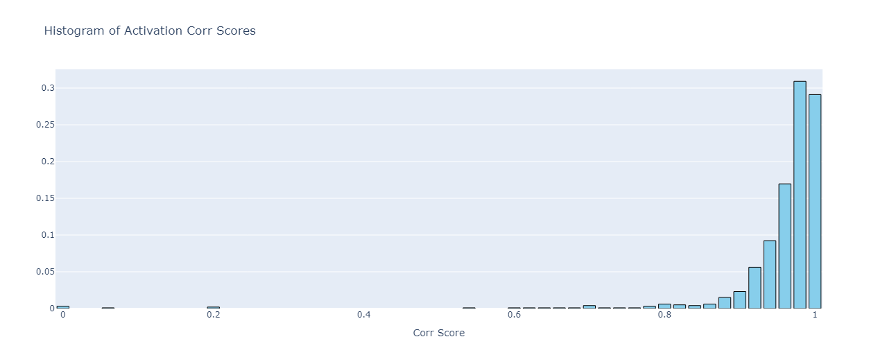
Moving on to the regular features, we expected to see a much more drastic dissimilarity of their activations. Indeed, the mean activation similarity for our sample of Gemma-2b regular feature is 0.39. Let’s check the histogram of these similarity scores:

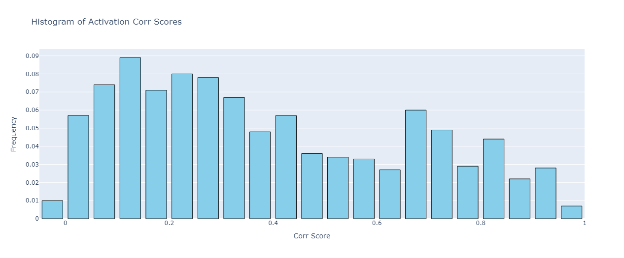
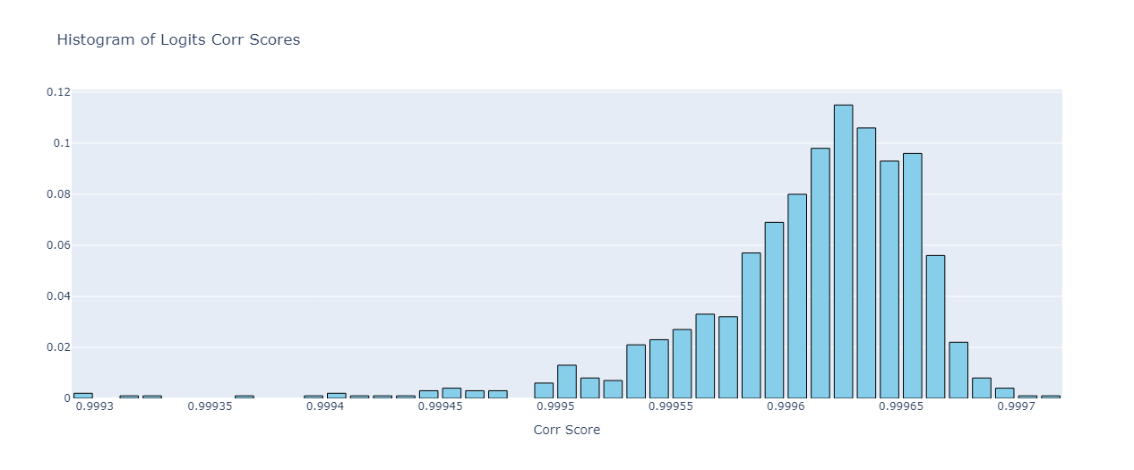
Interestingly, we see that a small fraction of features (~10%) have an activation similarity above 0.8! This implies that if these features were interpretable in the base model, they will most likely stay interpretable in the finetune modelWe didn’t try to manually interpret these features’ activations to verify this claim, and it would be interesting to see future works in this direction. But we’re not sure about the significance of this result: this could just as well be noise, so we invite further research in this area.

As for the logit similarity of these regular features, it turns out it’s much higher than our activation similarity, with a mean value of 0.952. Looking at the logit similarity scores histogram, it’s also much more concentrated towards the end of the interval:

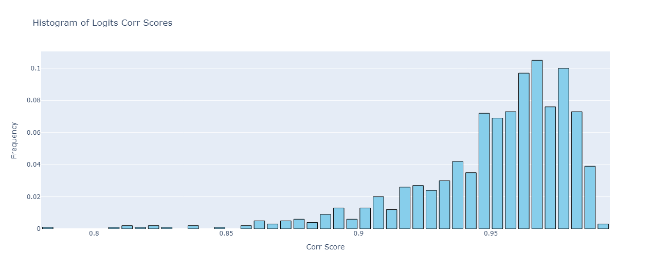
However, it’s easy to be misled by the mean logits similarity score. What it’s really saying is that our unembedding matrix (which is multiplied by the feature direction to get the logits similarity) hasn’t changed that much after finetuning (with a Frobenius norm ratio equal to 1.117 as we checked for our Gemma finetune). So if the feature has still the same direction, we can indeed say that the “direct feature effect” hasn’t changed in the finetuned model, but we never checked this premise! All we know is that there exist ~10% of features which have reasonably high activation similarity scores with the features from the base model. The key point is that the latter is a statement about the feature’s encoder direction (one that is used to project onto to get the feature’s activation, explained by Neel Nanda here), not the decoder one - which is what we mean when we talk about feature directions. So it could be the case that the feature is still there but changed its direction as discussed in this comment, it could also be that some features change their directions and the others don’t - it’s impossible to tell when the reconstruction score (e.g. variance explained) is as poor as in the Gemma-2b case.

5.3 Mistral-7B features transferability test

Here we repeat all the same experiments for Mistral-7B and its MetaMath finetune, and compare the result with the Gemma-2b case.

Let’s start with the features that are exclusively dead in the Mistral base model. Their mean activation error is 0.0003, which is almost two orders of magnitude lower than in the Gemma-2b case. The corresponding histogram looks like this:

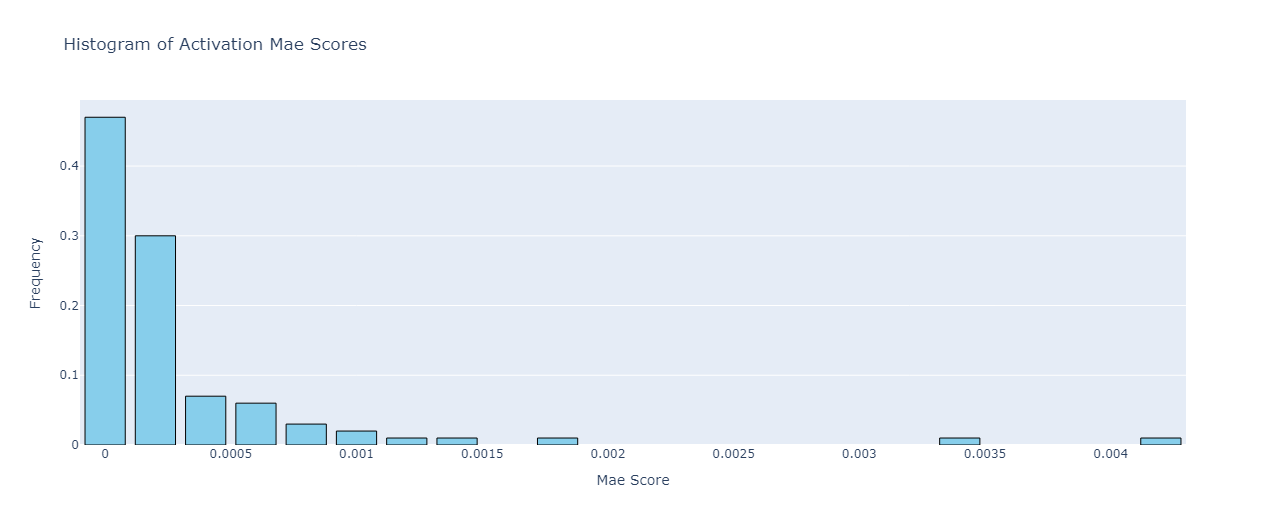
Once again, the results suggest that even though the dead features in the base model are no longer dead in the finetuned one, they activate really weakly on average, so it should be easy to adjust them with a cheap SAE finetuning.

The activation error for the features exclusively dead in the finetuned model tells a similar story:

Here the error is even smaller, implying that even though some features stopped activating after finetuning, their corresponding activation values in the base model were really low. And the features are often uninterpretable in the lowest activation intervals anyway, so it should have a minor overall effect on SAEs transferability.

Let’s conclude this section with an analysis of our regular features. As expected from the results of the last section, the activation similarity of these features is quite high, with a mean value of 0.958. As for the activation scores histogram:

As we can see, the distribution of the scores is strongly attracted to the 0.9-1.0 correlation interval, so we can conclude that SAE feature transferability is significantly high in this case. This is also backed up by the mean logits similarity of 0.9996, and a rather straightforward logits similarity histogram:

6. Conclusions & Limitations

6.1 Conclusions

Going back to our original question of “Do SAEs trained on a base model transfer to the finetuned one?”, the most obvious answer that comes to mind now is - it depends! We got drastically different results for our Gemma-2b-python-codes and Mistral-7B-MetaMath finetunes. However, it seems possible that one could estimate the “degree of transferability” in advance. One method is to compute various weight deviation metrics, such as the one used by Kissane et al for Gemma-2b, and another method that we used - to compute activation similarities of the model that are fed into an SAE. Both of these anecdotally correlate with the results of our transferability experiments, but a more thorough study is definitely needed.

Another takeaway we’ve had after finishing this post is that “SAE transferability” can mean different things. One can utilize the standard SAE evaluation metric to get a high-level evaluation of the SAE quality on the finetuned model, but it doesn’t always give a deeper insight into what happens with the SAE feature once we zoom in (which may be more interesting for the real SAE applications in mech interp). Our Gemma-2b results suggest that some SAE features may still be interpretable, even when finetuning has completely rendered the SAE incapable of reconstructing the input. And although the significance of this result can be rightly questioned, we still think it is interesting to investigate further.

6.2 Limitations

The main limitations we see in our work are the following:

It’s not clear how our results will generalize to other finetunes. A more principled approach would be to use a custom finetuning setup, where one could e.g. study the relationship between the amount of compute put into finetuning and some key SAE transferability metrics like the reconstruction loss etc.
- Our finetuned models also had almost the same dictionaries as the base model (with the exception of a single padding token), so it’s also not clear whether our results generalize to the finetuned model with significantly modified dictionaries (e.g. language finetunes for languages that were not in the original training dataset of the base model)
We only studied SAEs for a single residual layer for Gemma-2b and Mistral-7B models. A more thorough study is needed to see how these results will vary when considering different layers and different SAE activations, e.g. MLP or hidden head activations.
All our experiments were performed on the training dataset of the base SAE, i.e. on the original training distribution of the base models. But the finetuned models are mostly used for tasks that they have been finetuned on, so we definitely need some future work here to extend these results to a more specific setting of finetuned models.
Our analysis of SAE features transferability was somewhat superfluous, because we didn’t do a thorough investigation of the interpretability of our features after the finetuning. An even more representative study would be to replicate some kind of circuit analysis in the SAE basis to rigorously prove if (at least some) features are still involved in the same computation of the finetuned model.

Appendix

All code is available on github