Understanding Adversarial Vulnerabilities and Emergent Patterns in Multimodal RL
Using a simplified multimodal RL agent to explore adversarial vulnerabilities that emerge when using different modalities.
Introduction
Deep learning systems were once tailored to a single input type, for instance RGB pixels in image models
With that momentum comes a pressing need to evaluate how these systems handle adversarial pressure. Every deep learning stack depends on trust, especially when it supports safety critical decisions. We must understand how attackers can exploit multimodal pipelines and how the interaction between modalities shapes new strengths and new points of failure. While single modality models have a long history of research on perturbations and data poisoning, the community still has only partial visibility into how those threats appear when modalities overlap.
Live reinforcement learning agents raise the stakes even further. These policies operate within dynamic environments rather than static classification tasks, so defenses must respect timing, feedback, and control constraints. They also learn without labeled supervision, which complicates how we adapt classic adversarial tooling.
Exploring the impact of these attacks on multimodal reinforcement learning is of critical importance because these agents also see use in high risk robotics and autonomous platforms. A brittle policy in those domains risks severe safety incidents and expensive hardware failures.
Our study aims to map the interplay between adversarial attacks, defense strategies, and modality combinations on a baseline multimodal reinforcement learning agent. We document baseline performance and walk through empirical findings that show how different modality pairings shift behavior when attacked jointly or separately. We highlight how influence varies by modality and how defensive choices reshape those dynamics when interacting with different modalities.
To support this investigation we extend open-source code provided by authors of DDiffPG to create and release a full pipeline to prepare datasets, train reference models, and evaluate attack and defense mixes across modalities.
In this blog post we’ll talk about:
- Providing a testbed for adversarial evaluation of a multi-modal RL agent.
- Characterizing how attacking one or both modalities changes behavior.
- Showing that defenses introduce emergent patterns across modalities, sometimes improving robustness and sometimes destabilizing policies.
Background & Related Works
Research on adversarial robustness has largely centered on language and vision systems, especially as large language models expanded into multimodal applications such as text to image and image to text experiences
As embodied agents gain capability and broader deployment, we need a clearer view of how combined modalities influence security. Building resilient multimodal pipelines is essential for maintaining trust in systems that operate in high risk settings with steadily increasing task complexity.
Adversarial Attacks
Adversarial attacks are a branch of machine learning focused on manipulating model behavior in unintended or harmful ways. In particular, adversarial attacks are aimed at a “victim” model often designed with the flaws of a particular type of model or architecture in mind. These attacks typically involve introducing carefully designed “perturbations” to the input, which are intended to mislead or alter the model’s outputs. Depending on the attacker’s level of access to the internals of the model, attacks are classified as “white box” (full access, such as weights or gradient values), “gray box” (partial access, such as particular values or weights) or “black box” (no access at all, only inputs and outputs can be discerned around the black box). While perturbing inputs is the most common form of adversarial attack, other methods such as dataset “Poisoning” exist which alter training data to induce some desired behavior from the victim model.
Adversarial Attacks
Adversarial attacks are a critical area of study in modern machine learning, focusing on how models can be manipulated into producing incorrect or harmful outputs. These attacks exploit weaknesses in model architectures or training processes by introducing subtle, carefully designed perturbations to the input data. Although these changes are often imperceptible to humans, they can drastically alter a model’s predictions, revealing vulnerabilities in even the most sophisticated AI systems.
Types of Adversarial Attacks
Adversarial attacks are typically categorized based on the attacker’s level of access to the model’s internal information:
1. White-Box Attacks
In white-box attacks, the attacker has full access to the model’s internals, including parameters, gradients, and architecture details. This allows for precise and highly effective perturbations tailored to exploit specific weaknesses in the model.
2. Gray-Box Attacks
Gray-box attacks occur when the attacker has only partial access to the model. They may know certain weights, gradients, or architecture components, but not the entire system. These attacks are less direct than white-box methods but still capable of misleading models effectively.
3. Black-Box Attacks
In black-box attacks, the attacker has no insight into the model’s internal workings. They can only observe inputs and outputs, using this limited information to infer how to alter the input data. Black-box attacks often rely on query-based or transfer-based strategies to achieve success.
Beyond Input Perturbations: Data Poisoning
While most adversarial attacks occur during inference by altering input data, another powerful form of attack targets the training phase itself. Known as data poisoning, this method involves introducing manipulated samples into the training dataset. Over time, these poisoned samples bias the model’s learning process, leading to unintended or malicious behaviors once deployed.
Importance of Adversarial Robustness
As AI systems become increasingly integrated into critical domains such as healthcare, finance, and autonomous systems, ensuring their resilience to adversarial manipulation is essential. Developing models that can detect, resist, and adapt to these attacks is a cornerstone of building trustworthy, safe, and reliable machine learning applications.
Adversarial Defenses
Defending machine learning models against adversarial attacks is a multifaceted challenge that requires both proactive and reactive strategies. Broadly, adversarial defenses can be divided into three primary categories:
1. Adversarial Training
This approach involves augmenting the training process with adversarial samples
2. Attack and Anomaly Detection
Another common line of defense focuses on detecting adversarial activity by identifying perturbations, abnormal patterns, or suspicious data points before they can affect model performance
3. Input Filtering and Perturbation Removal
A third approach aims to remove or disrupt adversarial perturbations before the input reaches the model
Defense Methods Used in This Study
In our experiments, we employ three specific defense mechanisms aligned with the categories above:
- Disruption: Adding Gaussian noise to the input to reduce the impact of finely tuned perturbations.
- Detection: Utilizing a neural network classifier and traditional clustering techniques to identify anomalous inputs.
- Filtering: Applying a Variational Auto-Encoder (VAE) to reconstruct and denoise the input, effectively filtering out adversarial artifacts.
Together, these methods provide complementary layers of protection, enhancing the overall robustness of the model against diverse forms of adversarial interference.
Soft Actor-Critic Models
Soft Actor-Critic (SAC)
What makes SAC “soft” compared to traditional Actor-Critic methods is its inclusion of an entropy term in the objective function. This encourages the policy to remain more stochastic during training, promoting exploration rather than premature convergence to sub-optimal behaviors. In effect, SAC balances learning performance with policy diversity, achieving both stability and efficiency in complex, high-dimensional environments.
Methodology
Agent
To establish a baseline, we train a Soft Actor-Critic (SAC) agent
The agent’s observation space captures a comprehensive set of physical states to guide its behavior. It includes a velocity modality that records both linear and angular velocities (in meters and radians per second, respectively) for every limb, joint, and link of the Ant. Complementing this, an angular modality tracks joint angles in radians, covering the orientation between each limb link, the relative angles of the limbs to the torso, and the overall torso orientation.
In addition, the agent receives a z-coordinate reading representing the torso’s height above the ground in meters. Notably, all observations are unbounded, formally defined within the continuous range (-∞, ∞), allowing unrestricted representation of the agent’s motion dynamics.
The detailed observation space is outlined in the table below:
| Num | Observation | Name | Joint | Unit |
|---|---|---|---|---|
| 0 | z-coordinate of the torso (centre) | torso | free | position (m) |
| 1 | x-orientation of the torso (centre) | torso | free | angle (rad) |
| 2 | y-orientation of the torso (centre) | torso | free | angle (rad) |
| 3 | z-orientation of the torso (centre) | torso | free | angle (rad) |
| 4 | w-orientation of the torso (centre) | torso | free | angle (rad) |
| 5 | angle between torso and front left link on front left | hip_1 (front_left_leg) | hinge | angle (rad) |
| 6 | angle between the two links on the front left | ankle_1 (front_left_leg) | hinge | angle (rad) |
| 7 | angle between torso and front right link on front right | hip_2 (front_right_leg) | hinge | angle (rad) |
| 8 | angle between the two links on the front right | ankle_2 (front_right_leg) | hinge | angle (rad) |
| 9 | angle between torso and back left link on back left | hip_3 (back_left_leg) | hinge | angle (rad) |
| 10 | angle between the two links on the back left | ankle_3 (back_left_leg) | hinge | angle (rad) |
| 11 | angle between torso and back right link on back right | hip_4 (right_back_leg) | hinge | angle (rad) |
| 12 | angle between the two links on the back right | ankle_4 (right_back_leg) | hinge | angle (rad) |
| 13 | x-coordinate velocity of the torso | torso | free | velocity (m/s) |
| 14 | y-coordinate velocity of the torso | torso | free | velocity (m/s) |
| 15 | z-coordinate velocity of the torso | torso | free | velocity (m/s) |
| 16 | x-coordinate angular velocity of the torso | torso | free | angular velocity (rad/s) |
| 17 | y-coordinate angular velocity of the torso | torso | free | angular velocity (rad/s) |
| 18 | z-coordinate angular velocity of the torso | torso | free | angular velocity (rad/s) |
| 19 | angular velocity of the angle between torso and front left link | hip_1 (front_left_leg) | hinge | angle (rad) |
| 20 | angular velocity of the angle between front left links | ankle_1 (front_left_leg) | hinge | angle (rad) |
| 21 | angular velocity of the angle between torso and front right link | hip_2 (front_right_leg) | hinge | angle (rad) |
| 22 | angular velocity of the angle between front right links | ankle_2 (front_right_leg) | hinge | angle (rad) |
| 23 | angular velocity of the angle between torso and back left link | hip_3 (back_left_leg) | hinge | angle (rad) |
| 24 | angular velocity of the angle between back left links | ankle_3 (back_left_leg) | hinge | angle (rad) |
| 25 | angular velocity of the angle between torso and back right link | hip_4 (right_back_leg) | hinge | angle (rad) |
| 26 | angular velocity of the angle between back right links | ankle_4 (right_back_leg) | hinge | angle (rad) |
Table: Observations space for the MuJoCo Ant-Maze task. Ranges for all values are -Inf to +Inf.
The action space consists of 8 torque values applied to the rotors:
| Num | Action | Name | Joint | Type (Unit) |
|---|---|---|---|---|
| 0 | Torque applied on the rotor between the torso and back right hip | hip_4 (right_back_leg) | hinge | torque (N m) |
| 1 | Torque applied on the rotor between the back right two links | angle_4 (right_back_leg) | hinge | torque (N m) |
| 2 | Torque applied on the rotor between the torso and front left hip | hip_1 (front_left_leg) | hinge | torque (N m) |
| 3 | Torque applied on the rotor between the front left two links | angle_1 (front_left_leg) | hinge | torque (N m) |
| 4 | Torque applied on the rotor between the torso and front right hip | hip_2 (front_right_leg) | hinge | torque (N m) |
| 5 | Torque applied on the rotor between the front right two links | angle_2 (front_right_leg) | hinge | torque (N m) |
| 6 | Torque applied on the rotor between the torso and back left hip | hip_3 (back_leg) | hinge | torque (N m) |
| 7 | Torque applied on the rotor between the back left two links | angle_3 (back_leg) | hinge | torque (N m) |
Table: MuJoCo Ant agent action space. All values range between [-1, 1].
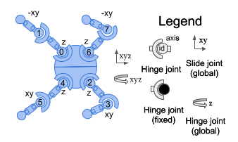
Below is an illustration of the body and rotor layout used in our experiments:

Environment
In addition to training the agent to embody its quadruped ant, we train it for the AI Gymnasium task “Ant Maze”
Adversarial Attack
We rely on the Fast Gradient Sign Method (FGSM)
- $\mathbf{x}$: The original input provided to the model.
- $y$: The true (ground-truth) label associated with the input.
- $\epsilon$: A small scalar value that controls the magnitude of the perturbation applied to the input.
- $J(\theta, \mathbf{x}, y)$: The loss function, parameterized by model weights $\theta$, input $\mathbf{x}$, and label $y$.
- $\nabla_{\mathbf{x}} J(\theta, \mathbf{x}, y)$: The gradient of the loss function with respect to the input, indicating how changes in $\mathbf{x}$ affect the loss.
- $\mathrm{sign}(\cdot)$: The element-wise sign function that extracts the direction (positive or negative) of each gradient component.
- $\mathbf{x}_{\text{adv}}$: The resulting adversarial example, formed by perturbing the original input $\mathbf{x}$ to maximize the model’s prediction error.
Modifying FGSM
FGSM is typically employed as an attack against image classifiers and perturbations are often in the form of pixel values. To get this to work in our case, we have to apply similar perturbations in the vector form matching our observation space. So we modify perturbations to represent values relative to which modality is being targeted (such as radians or meters per second).
The Fast Gradient Sign Method (FGSM) is traditionally designed for supervised learning tasks, particularly in classification, where each input is paired with a corresponding label. In such cases, the attack relies on the loss function, which depends on the model parameters, input, and true label. However, applying FGSM directly to reinforcement learning (RL) models presents a unique challenge, as RL agents often don’t use labeled data.
To address this, we reformulate FGSM in the following way. Instead of using a label-based loss, we leverage the critic’s Q-value as the optimization target. The modified FGSM equation is expressed as:
Here, the Q-function from the critic network replaces the conventional loss function. This adaptation enables FGSM to generate adversarial perturbations that specifically target the policy’s valuation process, influencing how the agent perceives the consequences of its actions. By perturbing inputs based on the critic’s gradients, we effectively reorient the attack for any unsupervised evaluation the critic is capable of.
Adversarial Defenses
Our evaluation includes three defense themes. We start with a disruption baseline that applies scaled gaussian noise to the observation vector. We then explore adversarial detection by training classifiers to flag perturbed observations and compare them with traditional clustering tools such as K Means and Gaussian Mixture Models (GMM). Finally, we assess a purification pipeline built on a defense VAE that reconstructs benign versions of the inputs.
Both the neural network detectors and the clustering approaches rely on a dataset collected during SAC training and evaluation. The agent runs for three million steps. We treat the first one point five million steps as a warm up phase to avoid logging data from an agent that has not yet learned to move reliably. During the final 1.5 million steps we record observations into a benign dataset. We also generate a matching adversarial dataset by applying FGSM perturbations to those observations without feeding the altered signals back to the agent. The result is a paired corpus of benign and adversarial samples for every modality.
Gaussian Noise Defense
The gaussian noise filter serves as the baseline defense. We sample perturbations from a normal distribution and scale them by $\epsilon$:
Targeted adversarial perturbations are often sensitive to small changes. By injecting a modest level of noise we can disrupt their structure and blunt the attack, accepting some degradation from the added randomness. This approach is simple and computationally inexpensive.
Defense VAE
Our defense VAE follows prior work on variational autoencoder purification
We adapt the architecture from image defenses to match our one dimensional observation vector. The compact network uses four fully connected layers with ReLU activation rather than convolutional stacks. Since the modalities are not arranged as a sequence with positional structure, we also avoid one dimensional convolutions.
Adversarial Detection
Detection centric defenses focus on identifying an attack rather than intervening directly in the control loop. We therefore evaluate them on prediction accuracy and F1 score but do not alter the agent mid run. A production system could take many actions once an attack is detected, yet that follow up is outside the scope of this study.
Using the labeled dataset we train Support Vector Machines (SVM), K Nearest Neighbors, and neural network classifiers to distinguish benign from adversarial observations. For comparison we also fit simpler clustering approaches such as K means and Gaussian Mixture Models to the same data.
Classifier accuracy reflects binary predictions on benign versus adversarial inputs. For the unsupervised clustering methods we assign cluster labels to maximize accuracy after fitting the two cluster model.
Adversarial Evaluation
We use the following process to test the effects of adversarial attacks on different modalities of our baseline agent:
- The agent is trained normally on benign inputs.
- Every evaluation episode, the input is perturbed with an attack: First across both modalities simultaneously, then focused on only target modalities in the agent’s observation.
- Compare adversarial evaluation to benign training performance and identify effects of the attack on the agent.
To better understand how defenses influence model performance, each defense method is tested under two different setups. In the first setup, the model is trained normally, and the defense is applied only during evaluation (filtering or otherwise “Defending” the input before it reaches the model). In the second setup, the model is also exposed to the defense during training by processing benign inputs through the same method before learning. The model is then attacked in the usual way. Comparing these two configurations reveals how much model tuning contributes to each defense’s effectiveness.
Results
Baseline Performance
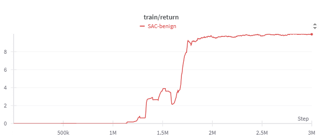
We begin by training an SAC agent on the Ant Maze task for three million steps so that it reliably clears a simple obstacle. The configuration mirrors common SAC settings with a replay buffer of one million transitions, $\tau=0.05$, and $\gamma=0.99$.
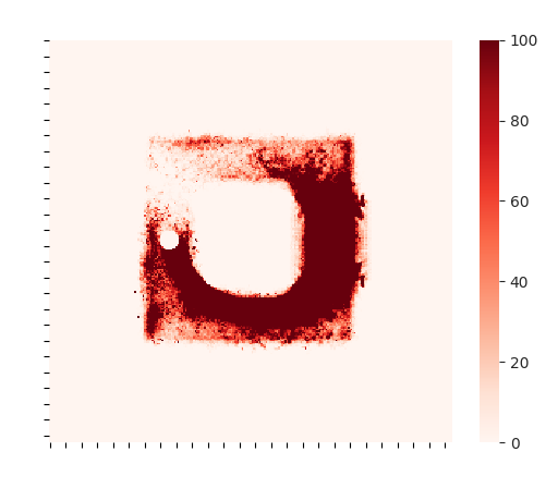
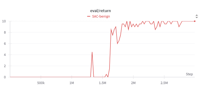
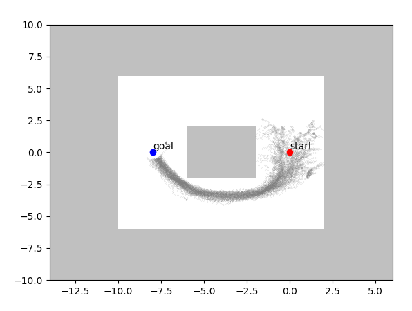
The figures below trace the training story. Rewards rise and level off after the run, the exploration heatmap shows how the agent learns an efficient route, and evaluation rewards peak once the policy stabilizes. The path visual confirms that the agent reaches the goal consistently.
With no adversarial pressure this baseline agent handles the maze it was trained on.
Attacking an Un-Defended Model
With the modified FGSM attack ($\epsilon=0.005$) we perturb the observation vector during evaluation. The attack seeks the lowest value outcome predicted by the critic, pushing the policy toward poor decisions.
Attacking Both Modalities
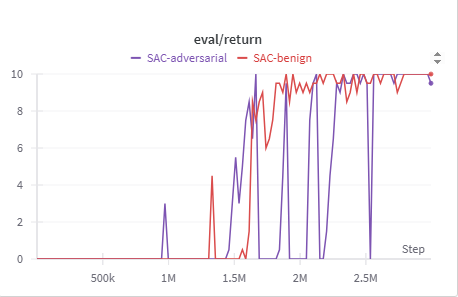
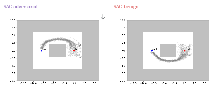
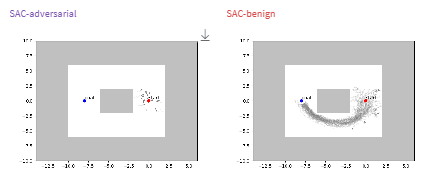
When we perturb both modalities, reward traces reveal the story immediately. Sharp drops in the purple line show successful attacks, while quick recoveries indicate attack attempts that did not succeed. The path comparisons illustrate what those swings look like in the environment: a failed attack nudges the agent onto an alternate route, whereas a successful one leaves the agent wandering near the start.
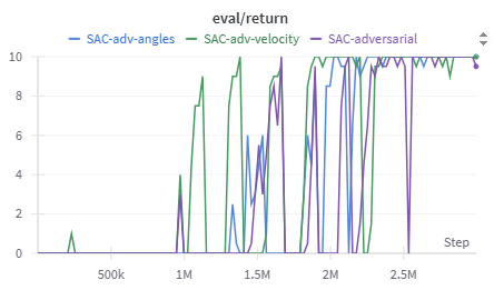
Attacking Individual Modalities
We then target each modality on its own with FGSM. The performance plot highlights how velocity (green) and angle (blue) perturbations differ from the full multimodal attack. Velocity covers roughly one quarter of the observation vector, so those attacks fail more often and produce more consistant reward. Angle perturbations cover more of the observation and are proportionally more effective.
These results reinforce a practical takeaway: the share of the observation space tied to a modality limits how much damage an attacker can cause when only that modality is manipulated. However this has potential to change on different systems, if an agent is severely biased towards using a single modality.
Modality-specific FGSM shows that attack effectiveness scales with the attacked fraction of the observation space.
Attacking a Defended Model
With the baseline established, we introduce defenses to see how they reshape the interaction between attacker and agent.
Gaussian Noise Defense
The gaussian noise filter is the simplest option. We add noise drawn from a normal distribution with mean zero and standard deviation one, scaled by 0.005.
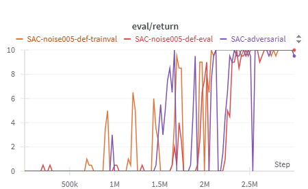
As shown in the noise defense results, even small amounts of injected noise can significantly disrupt the adversarial attack, leading to higher rewards during evaluation. Training the model with noise further improves its resilience, helping it adapt to the presence of randomness and reducing the attack’s overall success rate. In this setup, we evaluate two conditions: one where the model encounters noise only during evaluation, and another where it is pre-trained on noisy data.
Both approaches, training with noise (orange line) and applying noise only during evaluation (red line), show clear improvements compared to the undefended model (purple line). The trained model in particular exhibits more frequent reward peaks and fewer sharp drops, indicating that controlled noise not only weakens the attacker’s influence but also enhances the model’s overall stability under adversarial conditions.
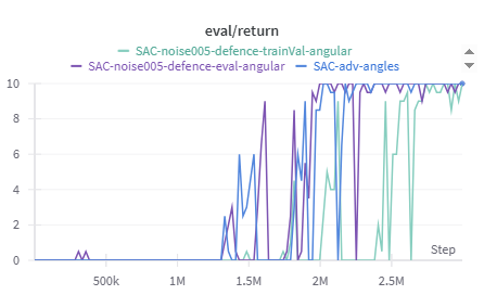
When applying Gaussian noise defenses to attacks targeting specific modalities, an interesting shift in behavior emerges. For velocity-targeted attacks, the results closely mirror those of the full multimodal noise defense, showing that noise effectively mitigates the attack’s impact. However, when the angular modality is targeted, the pattern changes noticeably.
In this case, training the model on noisy angular data appears to destabilize performance rather than improve it. The angular noise defense results show that the best-performing configuration occurs when noise is introduced only during evaluation, without exposing the model to it during training. The reason for this discrepancy remains unclear, it may be related to the angular modality’s dominant influence within the observation space, or potentially other underlying interactions in the model’s learning dynamics. Regardless, this behavior was observed consistently across multiple runs, suggesting a modality-specific sensitivity to noise based defenses.
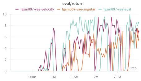
Defense-VAE
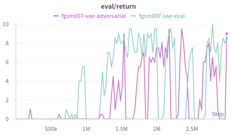
The compact Defense VAE offers another perspective. Running it only during evaluation lifts rewards under FGSM, but training the agent on VAE filtered inputs prevents the policy from solving the task. Single modality attacks expose its weaknesses: the VAE performs best when both modalities are perturbed together (as seen with the blue line in the figure below) and struggles with narrow attacks.
This pattern alligns with how the VAE learned. Training on paired benign and adversarial samples covering the entire observation space primes it to recognize broad perturbations. Once the attacker focuses on a single modality the reconstruction no longer matches the training distribution, so protection fades.
Detection Results (Summary)
The classifier roundup shows a clear trend: higher $\epsilon$ values (stronger perturbations) make detection easier. Angular perturbations are more detectable in general, and stand out at $\epsilon=0.007$, while velocity attacks become more visible at $\epsilon=0.015$. However clustering baselines such as K means and GMM hover near chance overall.
The broader lesson is that modality combinations shift detection difficulty, and scaling the attack changes that balance even when success rates stay similar.
The detailed results for all detection methods are shown in the table below:
| Detection Method | Multi-modal | Velocity | Angular | ||||||
|---|---|---|---|---|---|---|---|---|---|
| Accuracy | F1 Score | Epsilon | Accuracy | F1 Score | Epsilon | Accuracy | F1 Score | Epsilon | |
| SVM | 0.6027 | 0.6936 | 0.007 | 0.4993 | 0.6227 | 0.007 | 0.5606 | 0.6596 | 0.007 |
| SVM | 0.7188 | 0.7608 | 0.015 | 0.6070 | 0.7012 | 0.015 | 0.5048 | 0.3782 | 0.015 |
| KNN | 0.5909 | 0.5897 | 0.007 | 0.5164 | 0.4718 | 0.007 | 0.5391 | 0.5412 | 0.007 |
| KNN | 0.6606 | 0.6522 | 0.015 | 0.5850 | 0.5769 | 0.015 | 0.5152 | 0.3962 | 0.015 |
| NN | 0.7349 | 0.725 | 0.007 | 0.5494 | 0.6437 | 0.007 | 0.7104 | 0.7372 | 0.007 |
| NN | 0.9892 | 0.9892 | 0.015 | 0.8766 | 0.8810 | 0.015 | 0.8211 | 0.8264 | 0.015 |
| GMM | 0.4989 | N/A | 0.007 | 0.4984 | N/A | 0.007 | 0.4996 | N/A | 0.007 |
| GMM | 0.5094 | N/A | 0.015 | 0.4976 | N/A | 0.015 | 0.5021 | N/A | 0.015 |
| Kmeans | 0.5033 | N/A | 0.007 | 0.4998 | N/A | 0.007 | 0.5026 | N/A | 0.007 |
| Kmeans | 0.5416 | N/A | 0.015 | 0.4602 | N/A | 0.015 | 0.4855 | N/A | 0.015 |
Table: Classifier performance across modalities with FGSM epsilon (scaling) values of 0.007 and 0.015.
Conclusions
Our experiments confirm that a multimodal agent can be pushed off course through attacks on any of its inputs. The larger a modality’s footprint in the observation vector, the more influence an attacker gains. Defenses shape those dynamics in different ways: gaussian noise offers broad value with modality specific caveats, and the Defense VAE excels when the attack distribution matches its training data, even though the VAE is supposed to generalize well against new attack types/methods, it does not generalize as well across modalities.
These findings underline the importance of viewing reinforcement learning robustness through a modality aware lens. Simple interventions already reveal nuanced behavior, and the pipeline we release provides a starting point for deeper explorations.
The baseline setup here is intentionally lightweight, yet it highlights clear research directions for more complex agents and environments. We hope the insights and tools accelerate progress on safeguarding the next wave of multimodal systems.
Reproducibility Details
Experiments used SAC with 3M steps, replay size 1e6, $\tau=0.05$, $\gamma=0.99$, evaluation every 100 steps, and Adam learning rates as in our code. Defense-VAE used fully connected enc/dec layers (256-128-64 latent-64-128-256) with latent size 24, trained for 50 epochs. Classifier details and additional hyperparameters are available in the appendix of the paper and our codebase.
SAC Hyperparameters
| Parameter | Value |
|---|---|
| Horizon Length | 1 |
| Memory Size | $1 \times 10^6$ |
| Batch Size | 4096 |
| $N$-step | 1 |
| $\tau$ (Target smoothing coefficient) | 0.05 |
| $\gamma$ (Discount factor) | 0.99 |
| Warm-up Steps | 32 |
| Critic Class | Double Q-Network |
| Evaluation Frequency | 100 |
| Learning Rate (Alpha) | 0.005 |
| Update Times per Step | 8 |
VAE Hyperparameters
| Parameter | Value |
|---|---|
| Optimizer | Adam |
| Learning Rate | $1 \times 10^{-3}$ |
| Batch Size | 32 |
| Training Epochs | 50 |
| Latent Dimension | 24 |
| Encoder Layers | 5 (Observation, 256, 128, 64, Latent Dimension) |
| Decoder Layers | 5 (Latent Dimension, 64, 128, 256, Observation) |
Neural Network Hyperparameters
| Parameter | Value |
|---|---|
| Input Dimension | 28 |
| Output Dimension | 1 |
| Hidden Layers | 5 (256, 256, 128, 32, 1) |
| Learning Rate | 0.0001 |
| Training Epochs | 60 |
Support Vector Machine (SVM) Hyperparameters
| Parameter | Value |
|---|---|
| $C$ | 1000 |
| Gamma | 1 |
| Degree | 3 |
| Decision Function | One-vs-One (ovo) |
GMM Hyperparameters
| Parameter | Value |
|---|---|
| Number of Components | 2 |
| Initialization Method | k-means++ |
| Covariance Type | full |
| Convergence Tolerance ($\texttt{tol}$) | 0.001 |
| Regularization of Covariance ($\texttt{reg_covar}$) | $1 \times 10^{-6}$ |
| Max Iterations | 100 |
| Number of Initializations ($\texttt{n_init}$) | 1 |
K-Means
K-Means clustering algorithm as implemented by Scikit-learn, with a k value of 2 clusters.